Bag of features 图像检索

（一）数据集：

（二）SIFT特征简介：

1.1算法简介：

尺度不变特征转换即SIFT (Scale-invariant feature transform)是一种计算机视觉的算法。它用来侦测与描述影像中的局部性特征，它在空间尺度中寻找极值点，并提取出其位置、尺度、旋转不变量。
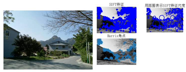
局部影像特征的描述与侦测可以帮助辨识物体，SIFT特征是基于物体上的一些局部外观的兴趣点而与影像的大小和旋转无关。对于光线、噪声、些微视角改变的容忍度也相当高。基于这些特性，它们是高度显著而且相对容易撷取，在母数庞大的特征数据库中，很容易辨识物体而且鲜有误认。使用 SIFT特征描述对于部分物体遮蔽的侦测率也相当高，甚至只需要3个以上的SIFT物体特征就足以计算出位置与方位。在现今的电脑硬件速度下和小型的特征数据库条件下，辨识速度可接近即时运算。SIFT特征的信息量大，适合在海量数据库中快速准确匹配。

实质：归为不同尺度空间上查找特征点（关键点）的问题。

1.2 SIFT算法实现特征匹配的主要三个步骤：

构建DOG尺度空间
关键点搜索和定位
方向赋值和特征描述的生成

1.3 实现结果：

（三）学习 “视觉词典”

1.1 对于一个庞大的数据集，可以通过聚类算法构建出视觉词典，聚类是实现 visual vocabulary /codebook的关键，最常用的就是K-means算法，算法流程:

• 随机初始化 K 个聚类中心
• 重复下述步骤直至算法收敛:

对应每个特征，根据距离关系赋值给某个中心/类别
对每个类别，根据其对应的特征集重新计算聚类中心

1.2 生成代码所需要的模型文件

生成视觉词典：

# -*- coding: utf-8 -*-
import pickle
from PCV.imagesearch import vocabulary
from PCV.tools.imtools import get_imlist
from PCV.localdescriptors import sift
##要记得将PCV放置在对应的路径下
#获取图像列表
imlist = get_imlist('D:/Visual_Studio_Code/data/first1000/') ###要记得改成自己的路径
nbr_images = len(imlist)
#获取特征列表
featlist = [imlist[i][:-3]+'sift' for i in range(nbr_images)]
#提取文件夹下图像的sift特征
for i in range(nbr_images):
    sift.process_image(imlist[i], featlist[i])
#生成词汇
voc = vocabulary.Vocabulary('ukbenchtest')
voc.train(featlist, 1000, 10)
#保存词汇
# saving vocabulary
with open(r'D:\Visual_Studio_Code\data\first1000\vocabulary.pkl', 'wb') as f:
    pickle.dump(voc, f)
print ('vocabulary is:', voc.name, voc.nbr_words)

（四）关键词权重度量：TF-IDF算法原理

1.1 算法思想：
TF-IDF（term frequency–inverse document frequency，词频-逆向文件频率）是用于信息检索与文本挖掘的重要算法，其中TF用于度量关键词在文档中的重要性，IDF用于度量关键词在全文档中的重要性，即文档中某关键词的重要性，与它在当前文档中的频率成正比，而与包含它的文档数成反比。
TF-IDF的主要思想是，若一个关键词在一篇文档中出现的频率高，而在其他文档中很少出现，则该关键词可较好的反应当前文档的特征。

1.2 算法原理：

度量某文档和查询的相关性，最简单的方法是利用各查询关键词在该文档中出现的总词频（Term Frequency，TF）。具体地，对于包含M个关键词的w1, w2,…wn查询，各关键词在某文档中出现的频率分别为：TF(w1), TF(w2),…,TF(wM)，则该文档与查询的相关性为：TF(w1)+TF(w2)+…+TF(wM)。

某些关键词可能同时出现在多篇文档中，该类关键词的主题预测能力较弱，可见，仅使用TF不能很好的反应文档与查询的相关性。关键词的主题预测能力越强，在度量与文档的相关性时，其权重应该越大。也就是说，若某关键词在较少文档中出现，则该关键词的权重应该较高，如关键词原子能的权重大于应用的权重。因此，利用包含某关键词的文档数，修正仅用词频TF度量该关键词的权重。在信息检索领域，使用逆文本频率（Inverse Document Frequency， IDF）表示关键词的主题预测能力（权重），表示为：

其中D为全部文档数，DF(w)为包含关键词w的文档数。
利用IDF的思想，文档与查询的相关性计算由简单的词频求和，变为以IDF为权重的加权求和，即

1.3 TF-IDF与信息论：

一个查询中，每个关键词的权重应该反应其为查询提供的信息量，简单的方法就是，用关键词的信息量，作为它在查询中的权重，即

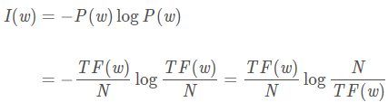其中N为整个语料库中的总词数，是可忽略的常数，此时：

若两个关键词在全文档中出现的频率相同，但第一个关键词集中分布在少数文章中，而第二个关键词分布在多篇文章中，显然，第一个关键词具有更好的主题预测能力，应赋予更高的查询权重。为此，提出以下假设（总文档数D，总词数N，包含关键词w的文档数DF(w)）：每个文档含词数基本相同，即

每个关键词一旦在文档中出现，不论其出现多少次，权重都相同，即关键词w在文档中未出现，则权重为0；否则，则为：

因此，关键词w的信息量

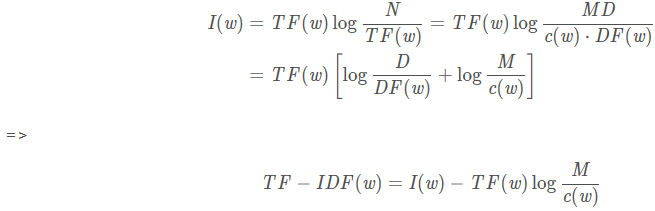易知，关键词w的TF-IDF值，与其信息量成正比；又由于M>c(w)，知关键词w的TF-IDF值，与其在文档中出现的平均次数成反比，这些结论完全符合信息论。

1.4 平滑处理：
经过平滑处理后, IDF的最终计算公式如下：

log项中分子项和分母项均加1，表示虚拟增加一篇包含任意词的文档，避免分母项为0；IDF的最终值加1，避免某单词在所有文档中出现时，IDF的值为0，即不忽略出现在所有文档中的词；

1.5 正则化处理：

sklearn中类TfidfTransformer默认对文档的TF-IDF特征向量做l2正则化，即某文档的TF-IDF特征向量为v，则

若单词表为{w1, w2, w3}，文档A=(w1, w2, w2)，B=(w1, w2, w3)，且w1, w2, w3的IDF值相同，则未正则化时，

此时，文档A、B中单词w1的TF-IDF值相同。若进行l2正则化，则

可见文档B中w1的TF-IDF值（权重）更大，正则化后的意义为：考虑文档的TF-IDF特征分布，增加不同权重之间的差异。不失一般性，文档A、B中正则化后w1的TF-IDF分别为

，如TF(A_w1) = TF(B_w1)，且TF之和为1，知

推导出

进而，推导出

当前仅当TF(B_w2) = 0或TF(B_w3) = 0，即B中w2或w3的频率为0时，等式成立。

1.6 算法实现：

算法的实现参考了sklearn.feature_extraction.text中的CountVectorizer和TfidfVectorizer类，如下：

import re
from collections import defaultdict

from sklearn.feature_extraction.text import CountVectorizer, TfidfVectorizer
import numpy as np
from scipy.sparse import csr_matrix, spdiags
from scipy.sparse.linalg import norm

PTN_SYMBOL = re.compile(r'[.!?\'",]')


def tokenize(doc):
    """
    英文分词，小写输出
    """
    for word in PTN_SYMBOL.sub(' ', doc).split(' '):
        if word and word != ' ':
            yield word.lower()


def count_vocab(raw_documents):
    """
    返回文档词频的稀疏矩阵
    参考sklearn.feature_extraction.text.CountVectorizer._count_vocab

    矩阵大小：M*N, M个文档, 共计N个单词
    :param raw_documents: ['Hello world.', 'Hello word', ...]
    :return: csc_matrix, vocabulary
    """
    vocab = {}
    data, indices, indptr = [], [], [0]

    for doc in raw_documents:
        doc_feature = defaultdict(int)
        for term in tokenize(doc):
            # 词在词表中的位置
            index = vocab.setdefault(term, len(vocab))
            # 统计当前文档的词频
            doc_feature[index] += 1
        # 存储当前文档的词及词频
        indices.extend(doc_feature.keys())
        data.extend(doc_feature.values())
        # 累加词数
        indptr.append(len(indices))

    # 构造稀疏矩阵
    X = csr_matrix((data, indices, indptr), shape=(len(indptr) - 1, len(vocab)), dtype=np.int64)

    # 将单词表排序，同时更新压缩矩阵数据的位置
    map_index = np.empty(len(vocab), dtype=np.int32)
    for new_num, (term, old_num) in enumerate(sorted(vocab.items())):
        vocab[term] = new_num
        map_index[old_num] = new_num
    X.indices = map_index.take(X.indices, mode='clip')

    X.sort_indices()

    return X, vocab


def tfidf_transform(X, smooth_idf=True, normalize=True):
    """
    将词袋矩阵转换为TF-IDF矩阵

    :param X: 压缩的词袋矩阵 M*N， 文本数M, 词袋容量N
    :param smooth_idf: 是否对DF平滑处理
    :param normalize: 是否对TF-IDF执行l2标准化
    :return: TF-IDF压缩矩阵(csc_matrix)
    """
    n_samples, n_features = X.shape

    df = np.bincount(X.indices, minlength=X.shape[1])
    df += int(smooth_idf)
    new_n_samples = n_samples + int(smooth_idf)
    idf = np.log(float(new_n_samples) / df) + 1.0

    # 对角稀疏矩阵N*N，元素值对应单词的IDF
    idf_diag = spdiags(idf, diags=0, m=n_features, n=n_features, format='csr')

    # 等价于 DF * IDF
    X = X * idf_diag

    # 执行l2正则化
    if normalize:
        norm_l2 = 1. / norm(X, axis=1)
        tmp = spdiags(norm_l2, diags=0, m=n_samples, n=n_samples, format='csr')
        X = tmp * X

    return X


if __name__ == '__main__':
    # 源文档
    raw_documents = [
        'This is the first document.',
        'This is the second second document.',
        'And the third one.',
        'Is this the first document?',
    ]
    # 转换为词袋模型
    X, vocab = count_vocab(raw_documents)
    # X = CountVectorizer().fit_transform(raw_documents)
    """
    >> vocab
    {'this': 8, 'is': 3, 'the': 6, 'first': 2, 'document': 1, 'second': 5, 'and': 0, 'third': 7, 
    'one': 4}
    
    >> X.toarray()
    [[0 1 1 1 0 0 1 0 1]
     [0 1 0 1 0 2 1 0 1]
     [1 0 0 0 1 0 1 1 0]
     [0 1 1 1 0 0 1 0 1]]
    """

    # 计算TF-IDF
    tfidf_x = tfidf_transform(X)
    # tfidf_x = TfidfVectorizer().fit_transform(raw_documents)
    """
    >> tfidf_x.toarray()
    [   [0.       0.439       0.542       0.439       0.          0.      0.359   0.         0.439]
        [0.       0.272       0.          0.272       0.          0.853   0.223   0.         0.272]
        [0.553    0.          0.          0.          0.553       0.      0.288   0.553      0.   ]
        [0.       0.439       0.542       0.439       0.          0.      0.359   0.         0.439]	]

1.7总结：

优点：简单快速，结果符合实际情况
缺点：单纯以词频衡量词的重要性，不够全面，有时重要的词出现的次数不多，而且对词的出现位置没有设置，出现位置靠前的词和出现位置靠后的词的重要性一样，可以对全文的第一段或者每一段的第一句给予较大的权重。首先将图像转化为特征向量在作为网络的输入，要远比图像直接作为网络输入的数据量要小得多。同时将图像使用网络模型特诊向量化时，也保留了图像的特征，不论在识别还是分类任务上，对最终实现的分类效果或识别效果影响不大？（可能我没追求那么多）而且不管向量压缩的维度至多少，只需将训练时输入网络和测试时输入网络的图像均转化为同一维度，使其在同一个向量空间中，神经网络就能通过优化器进行学习，

（五）基于内容的图像检索

1.1在大型图像数据库上，CBIR技术用于检索在视觉上具有相似性的图像。这样返回的图像可以是颜色相似，纹理相似，图像中的物体或场景相似；总之，基本上可以是这些图像自身共有的任何信息。
对于高层查询，比如寻找相似物体，将查询图像与数据库中所有的图像进行完全比较（比如用特征匹配）往往是不可行的。在数据库很大的情况下，这样的查询方式，会耗费过多的时间。在过去的几年时间里，研究者成功地引入了文本挖掘技术到CBIR中处理问题，使在百万图像中搜索具有相似内容的图像成为可能。

1.2 视觉单词

为了将文本挖掘技术应用到图像中，我们首先需要建立视觉等效单词；这通常可以采用SIFT局部描述子可以做到。它的思想是将描述子空间量化成一些典型实例，并将图像中的每个描述子指派到其中的某个实例中。这些典型实例可以通过分析训练图像集确定，并被视为视觉单词。所有这些视觉单词构成的集合称为视觉词汇。从一个图像集中提取特征描述子，利用一些聚类算法可以构建出视觉单词。聚类算法中最常用的是K-means。视觉单词是在给定特征描述子空间中的一组向量集，在采用K-means进行聚类时得到的视觉单词是聚类质心。用视觉单词直方图来表示图像，则该模型便称为BOW模型。

1.3特征提取

特征提取就是通过我们常用的sifi方法，提取图像的特征。

4. 针对输入特征集，根据视觉词典进行量化

对于输入特征，量化的过程是将该特征映射到距离其最接近的视觉单词，并实现计数。

5. 把输入图像，根据TF-IDF转化成视觉单词（visual words）的频率直方图

6.构造特征到图像的倒排表，通过倒排表快速索引相关图像

7.根据索引结果进行直方图匹配

1.4代码及结果实现

1、提取特征值：

#提取文件夹下图像的sift特征
for i in range(nbr_images):
    sift.process_image(imlist[i], featlist[i])

2、生成词汇字典/码本、

# -*- coding: utf-8 -*-
import pickle
from PCV.imagesearch import vocabulary
from PCV.tools.imtools import get_imlist
from PCV.localdescriptors import sift

#获取图像列表
imlist = get_imlist('E:/BaiduNetdiskDownload/PCV-book-data/data/first1000/')
nbr_images = len(imlist)
#获取特征列表
featlist = [imlist[i][:-3]+'sift' for i in range(nbr_images)]

#提取文件夹下图像的sift特征
for i in range(nbr_images):
    sift.process_image(imlist[i], featlist[i])

#生成词汇
voc = vocabulary.Vocabulary('ukbenchtest')
voc.train(featlist, 1000, 10)
#保存词汇
# saving vocabulary
with open('E:/BaiduNetdiskDownload/PCV-book-data/data/first1000/vocabulary.pkl', 'wb') as f:
    pickle.dump(voc, f)
print 'vocabulary is:', voc.name, voc.nbr_words

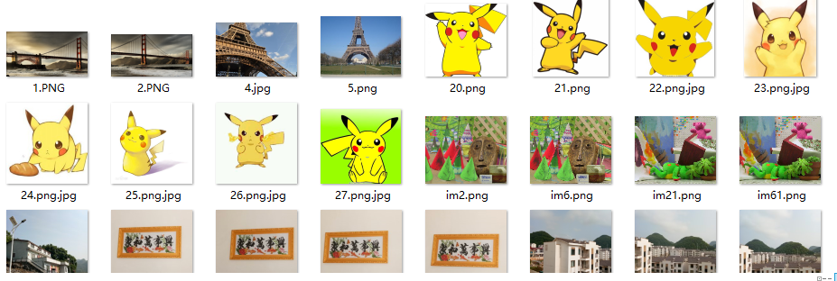
这里的图像使用的是first1000（肯塔基大学物体识别数据集前1000幅图像）。生成了图像的sift文件和码本
在这里插入图片描述

3、建立并将数据存入数据库

# -*- coding: utf-8 -*-
import pickle
from PCV.imagesearch import imagesearch
from PCV.localdescriptors import sift
from sqlite3 import dbapi2 as sqlite
from PCV.tools.imtools import get_imlist

#获取图像列表
imlist = get_imlist('./first1000/')
nbr_images = len(imlist)
#获取特征列表
featlist = [imlist[i][:-3]+'sift' for i in range(nbr_images)]

# load vocabulary
#载入词汇
with open('./first1000/vocabulary.pkl', 'rb') as f:
    voc = pickle.load(f)
#创建索引
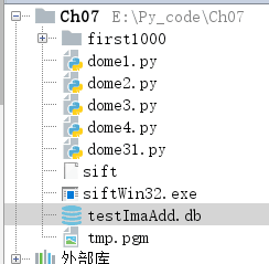
indx = imagesearch.Indexer('testImaAdd.db',voc)
indx.create_tables()
# go through all images, project features on vocabulary and insert
#遍历所有的图像，并将它们的特征投影到词汇上
for i in range(nbr_images)[:500]:
    locs,descr = sift.read_features_from_file(featlist[i])
    indx.add_to_index(imlist[i],descr)
# commit to database
#提交到数据库
indx.db_commit()

con = sqlite.connect('testImaAdd.db')
print con.execute('select count (filename) from imlist').fetchone()
print con.execute('select * from imlist').fetchone()

这一步会生成一个新的数据库，储存图像的数据
在这里插入图片描述

4、对图像检索

# -*- coding: utf-8 -*-
import pickle
from PCV.localdescriptors import sift
from PCV.imagesearch import imagesearch
from PCV.geometry import homography
from PCV.tools.imtools import get_imlist

# load image list and vocabulary
#载入图像列表
imlist = get_imlist('./first1000/')
nbr_images = len(imlist)
#载入特征列表
featlist = [imlist[i][:-3]+'sift' for i in range(nbr_images)]

#载入词汇
with open('./first1000/vocabulary.pkl', 'rb') as f:
    voc = pickle.load(f)

src = imagesearch.Searcher('testImaAdd.db',voc)

# index of query image and number of results to return
#查询图像索引和查询返回的图像数
q_ind = 0
nbr_results = 20

# regular query
# 常规查询(按欧式距离对结果排序)
res_reg = [w[1] for w in src.query(imlist[q_ind])[:nbr_results]]
print('top matches (regular):', res_reg)

# load image features for query image
#载入查询图像特征
q_locs,q_descr = sift.read_features_from_file(featlist[q_ind])
fp = homography.make_homog(q_locs[:,:2].T)

# RANSAC model for homography fitting
#用单应性进行拟合建立RANSAC模型
model = homography.RansacModel()
rank = {}

# load image features for result
#载入候选图像的特征
for ndx in res_reg[1:]:
    locs,descr = sift.read_features_from_file(featlist[ndx])  # because 'ndx' is a rowid of the DB that starts at 1
    # get matches
    matches = sift.match(q_descr,descr)
    ind = matches.nonzero()[0]
    ind2 = matches[ind]
    tp = homography.make_homog(locs[:,:2].T)
    # compute homography, count inliers. if not enough matches return empty list
    try:
        H,inliers = homography.H_from_ransac(fp[:,ind],tp[:,ind2],model,match_theshold=4)
    except:
        inliers = []
    # store inlier count
    rank[ndx] = len(inliers)

# sort dictionary to get the most inliers first
sorted_rank = sorted(rank.items(), key=lambda t: t[1], reverse=True)
res_geom = [res_reg[0]]+[s[0] for s in sorted_rank]
print('top matches (homography):', res_geom)

# 显示查询结果
imagesearch.plot_results(src,res_reg[:8]) #常规查询
imagesearch.plot_results(src,res_geom[:8]) #重排后的结果

5、通过常规查询和用单应性进行拟合建立RANSAC模型进行查询的结果如下

测试图片：

常规查询

总结：

总结的来说匹配效果是最好的，图片特征明显的和图片数量较多的，训练效果的好坏直接影响整个算法的识别正确率。而影响训练效果的因素主要有图片的数量和图片特征的差距，对于第二组实验如果有更多的数据集，对于其他人的匹配效果肯定也是和前两位的效果差不多。

————————————————

参考链接：
https://blog.csdn.net/sinat_34072381/article/details/89648124

https://blog.csdn.net/sinat_34072381/article/details/89648124

https://www.cnblogs.com/silencexiaoyou/p/10861735.html

posted @ 2020-05-24 22:23 cenyan 阅读(523) 评论(0) 收藏举报

刷新页面返回顶部

cenyan

Bag of features 图像检索

公告