金融量化分析

• 第一部分：金融与量化投资
• 第二部分：量化投资与Python
• 第三部分 实现简单的量化框架
• 第四部分 在线平台与量化投资

第一部分：金融与量化投资

股票：

• 股票是股份公司发给出资人的一种凭证，股票的持有者就是股份公司的股东。

股票的面值与市值

• 面值表示票面金额
• 市值表示市场价值

上市/IPO：

• 企业通过证券交易所公开向社会增发股票以募集资金

股票的作用：

• 出资证明、证明股东身份、对公司经营发表意见
• 公司分红、交易获利

股票的分类

股票按业绩分类：

• 蓝筹股：资本雄厚、信誉优良的公司的股票
• 绩优股：业绩优良公司的股票
• ST股：特别处理股票，连续两年亏损或每股净资产低于股票面值

股票按上市地区分类：

• A股：中国大陆上市，人民币认购买卖（T+1，涨跌幅10%）
• B股：中国大陆上市，外币认购买卖（T+1，T+3）
• H股：中国香港上市（T+0，涨跌幅不设限制）
• N股：美国纽约上市
• S股：新加坡上市

股票市场的构成

• 上市公司
• 投资者（包括机构投资者）
• 证监会、证券业协会、交易所
• 证券中介机构

交易所

• 上海证券交易所：只有一个主板（沪指）
• 深圳证券交易所：

1. 主板：大型成熟企业（深成指）
2. 中小板：经营规模较小
3. 创业板：尚处于成长期的创业企业

影响股价的因素

• 公司自身因素：股票自身价值是决定股价最基本的因素，而这主要取决于发行公司的经营业绩、资信水平以及连带而来的股息红利派发状况、发展前景、股票预期收益水平等。
• 行业因素：行业在国民经济中地位的变更，行业的发展前景和发展潜力，新兴行业引来的冲击等，以及上市公司在行业中所处的位置，经营业绩，经营状况，资金组合的改变及领导层人事变动等都会影响相关股票的价格。
• 市场因素：投资者的动向，大户的意向和操纵，公司间的合作或相互持股，信用交易和期货交易的增减，投机者的套利行为，公司的增资方式和增资额度等，均可能对股价形成较大影响。
• 心理因素：情绪波动，判断失误，盲目追随大户、狂抛抢购
• 经济因素：经济周期，国家的财政状况，金融环境，国际收支状况，行业经济地位的变化，国家汇率的调整等
• 政治因素

股票买卖（A股）

• 委托买卖股票 : 个人不能直接买卖，需要在券商开户，进行委托购买
• 股票交易日：周一到周五（非法定节假日和交易所休市日）
• 股票交易时间：
  • 9:15-9:25 开盘集合竞价时间
  • 9:30-11:30 前市，连续竞价时间
  • 13:00-15:00 后市，连续竞价时间
  • 14:57-15:00 深交所收盘集合竞价时间
• T+1交易制度：股票买入后当天不能卖出，要在买入后的下一个交易日才能卖出
• 涨停、跌停限制

金融分析

基本面分析

• 宏观经济面分析：国家的财政政策、货币政策等
• 行业分析
• 公司分析：财务数据、业绩报告等

技术面分析：各项技术指标

• K线
• MA（均线）
• KDJ（随机指标）
• MACD（指数平滑移动平均线）
• ……

K线

金融量化投资

• 量化投资：利用计算机技术并且采用一定的数学模型去实践投资理念，实现投资策略的过程。
• 量化投资的优势：
  • 避免主观情绪、人性弱点和认知偏差，选择更加客观
  • 能同时包括多角度的观察和多层次的模型
  • 及时跟踪市场变化，不断发现新的统计模型，寻找交易机会
  • 在决定投资策略后，能通过回测验证其效果

量化策略

• 量化策略：通过一套固定的逻辑来分析、判断和决策，自动化地进行股票交易。
• 核心内容
  •  选股
  • 择时
  • 仓位管理
  • 止盈止损
• 策略的周期
  • 产生想法/学习知识
  • 实现策略：Python
  • 检验策略：回测/模拟交易
  • 实盘交易
  • 优化策略/放弃策略

第二部分：量化投资与Python

量化投资与Python

• 为什么选择Python?
  • 其他选择：Excel、SAS/SPSS、R
• 量化投资第三方相关模块
  • NumPy：数值计算
  • pandas：数据分析
  • Matplotlib：图标绘制
• 如何使用Python进行量化投资
  • 自己编写：NumPy+pandas+Matplotlib+……
  • 在线平台：聚宽、优矿、米筐、Quantopian、……
  • 开源框架：RQAlpha、QUANTAXIS、……

Ipython:交互式的Python命令行

• IPython：安装：pip install ipython
• TAB键自动完成
• ?命令（内省、命名空间搜索）
• 执行系统命令（!）
• %run命令执行文件代码
• %paste %cpaste命令执行剪贴板代码
• 与编辑器和IDE交互
• 魔术命令：%timeit %pdb …
• 使用命令历史
• 输入与输出变量（_, __, _2, _i2）
• 目录书签系统 %bookmark
• Ipython Notebook

Ipython常用的魔术命令

 

 

Python调试器命令

Ipython快捷键

NumPy：数组计算

• NumPy是高性能科学计算和数据分析的基础包。它是pandas等其他各种工具的基础。
• NumPy的主要功能：
  • ndarray，一个多维数组结构，高效且节省空间
  • 无需循环对整组数据进行快速运算的数学函数
  • *读写磁盘数据的工具以及用于操作内存映射文件的工具
  • *线性代数、随机数生成和傅里叶变换功能
  • *用于集成C、C++等代码的工具
• 安装方法：pip install numpy
• 引用方式：import numpy as np

NumPy：ndarray-多维数组对象

• 创建ndarray：np.array()
• 为什么要使用ndarray：
  • 例1：已知若干家跨国公司的市值（美元），将其换算为人民币
  • 例2：已知购物车中每件商品的价格与商品件数，求总金额
• ndarray还可以是多维数组，但元素类型必须相同
• 常用属性：
  • T 数组的转置（对高维数组而言）
  • dtype 数组元素的数据类型
  • size 数组元素的个数
  • ndim 数组的维数
  • shape 数组的维度大小（以元组形式）

NumPy：ndarray-多维数组对象

• dtype：
  • bool_, int(8,16,32,64), uint(8,16,32,64), float(16,32,64)
  • 类型转换：astype()
• 创建ndarray：
  • array() 将列表转换为数组，可选择显式指定dtype
  • arange() range的numpy版，支持浮点数
  • linspace() 类似arange()，第三个参数为数组长度
  • zeros() 根据指定形状和dtype创建全0数组
  • ones() 根据指定形状和dtype创建全1数组
  • empty() 根据指定形状和dtype创建空数组（随机值）
  • eye() 根据指定边长和dtype创建单位矩阵

NumPy：索引和切片

• 数组和标量之间的运算
  • a+1 a*3 1//a a**0.5
• 同样大小数组之间的运算
  • a+b
  • a/b
  • a**b
• 数组的索引
  • a[5]
  • a2[2][3]
  • a2[2,3]
• 数组的切片
  • a[5:8]
  • a[:3] = 1
  • a2[1:2, :4]
  • a2[:,:1]
  • a2[:,1]
• 与列表不同，数组切片时并不会自动复制，在切片数组上的修改会影响原数组。
• b = a[:4]
• b[-1] = 250
• 解决方法：
• copy()】 b = a[:4] b[-1] = 250

NumPy：布尔型索引

• 问题：给一个数组，选出数组中所有大于5的数。
  • 答案：a[a>5]
  • 原理： a>5会对a中的每一个元素进行判断，返回一个布尔数组 布尔型索引：将同样大小的布尔数组传进索引，会返回一个由所有True对应位置的元素的数组
• 问题2：给一个数组，选出数组中所有大于5的偶数。
• 问题3：给一个数组，选出数组中所有大于5的数和偶数。
  • 答案： a[(a>5) & (a%2==0)] a[(a>5) | (a%2==0)]

NumPy：花式索引*

• 问题1：对于一个数组，选出其第1，3，4，6，7个元素，组成新的二维数组。
  • 答案：a[[1,3,4,6,7]]
• 问题2：对一个二维数组，选出其第一列和第三列，组成新的二维数组。
  • 答案：a[:,[1,3]]

NumPy：通用函数

• 通用函数：能同时对数组中所有元素进行运算的函数
• 常见通用函数：
  • 一元函数：abs, sqrt, exp, log, ceil, floor, rint, trunc, modf, isnan, isinf, cos, sin, tan
  • 二元函数：add, substract, multiply, divide, power, mod, maximum, mininum,

NumPy：数学和统计方法

• 常用函数：
  • sum 求和
  • mean 求平均数
  • std 求标准差 v
  • ar 求方差
  • min 求最小值
  • max 求最大值
  • argmin 求最小值索引
  • argmax 求最大值索引

NumPy：随机数生成

• 常用函数
  • rand 给定形状产生随机数组（0到1之间的数）
  • randint 给定形状产生随机整数
  • choice 给定形状产生随机选择
  • shuffle 与random.shuffle相同
  • uniform 给定形状产生随机数组

pandas：数据分析

• pandas是一个强大的Python数据分析的工具包。
• pandas是基于NumPy构建的。
• pandas的主要功能
  • 具备对其功能的数据结构DataFrame、Series
  • 集成时间序列功能
  • 提供丰富的数学运算和操作
  • 灵活处理缺失数据
• 安装方法：pip install pandas
• 引用方法：import pandas as pd

pandas：Series

• Series是一种类似于一位数组的对象，由一组数据和一组与之相关的数据标签（索引）组成。
  • Series比较像列表（数组）和字典的结合体
• 创建方式：
  • pd.Series([4,7,-5,3])
  • pd.Series([4,7,-5,3],index=['a','b','c','d'])
  • pd.Series({'a':1, 'b':2})
  • pd.Series(0, index=['a','b','c','d'])
• 获取值数组和索引数组：
  • values属性
  • index属性

pandas：Series特性

• Series支持NumPy模块的特性（下标）：
  • 从ndarray创建Series：Series(arr)
  • 与标量运算：sr*2
  • 两个Series运算：sr1+sr2
  • 索引：sr[0], sr[[1,2,4]]
  • 切片：sr[0:2]（切片依然是视图形式）
  • 通用函数：np.abs(sr)
  • 布尔值过滤：sr[sr>0]
  • 统计函数：mean() sum() cumsum()

pandas：整数索引

• 整数索引的pandas对象往往会使新手抓狂。
• 例：
  • sr = np.Series(np.arange(4.))
  • sr[-1]
• 如果索引是整数类型，则根据整数进行数据操作时总是面向标签的。
  •  loc属性 以标签解释
  • iloc属性 以下标解释

pandas：Series数据对齐

• pandas在运算时，会按索引进行对齐然后计算。如果存在不同的索引，则结果的索引是两个操作数索引的并集。
• 例：
  • sr1 = pd.Series([12,23,34], index=['c','a','d'])
  • sr2 = pd.Series([11,20,10], index=['d','c','a',])
  • sr1+sr2
  • sr3 = pd.Series([11,20,10,14], index=['d','c','a','b'])
  • sr1+sr3
• 如何在两个Series对象相加时将缺失值设为0？
  • sr1.add(sr2, fill_value=0)
  • 灵活的算术方法：add, sub, div, mul

pandas：Series缺失数据

• 缺失数据：使用NaN（Not a Number）来表示缺失数据。其值等于np.nan。内置的None值也会被当做NaN处理。
• 处理缺失数据的相关方法：
  • dropna() 过滤掉值为NaN的行
  • fillna() 填充缺失数据
  • isnull() 返回布尔数组，缺失值对应为True
  • notnull() 返回布尔数组，缺失值对应为False
• 过滤缺失数据：
  • sr.dropna()
  • sr[data.notnull()]
• 填充缺失数据：fillna(0)

pandas：DataFrame

• DataFrame是一个表格型的数据结构，含有一组有序的列。
• DataFrame可以被看做是由Series组成的字典，并且共用一个索引。
• 创建方式：
  • pd.DataFrame({'one':[1,2,3,4],'two':[4,3,2,1]})
  • pd.DataFrame({'one':pd.Series([1,2,3],index=['a','b','c']), 'two':pd.Series([1,2,3,4],index=['b','a','c','d'])})
  • ……
• csv文件读取与写入：
  • df.read_csv('filename.csv')
  • df.to_csv()

pandas：DataFrame查看数据

• 查看数据常用属性及方法：
  • index 获取索引
  • T 转置
  • columns 获取列索引
  • values 获取值数组
  • describe() 获取快速统计
• DataFrame各列name属性：列名
  • rename(columns={})

pandas：DataFrame索引和切片

• DataFrame有行索引和列索引。
• 通过标签获取：
  •  df['A']
  • df[['A', 'B']]
  • df['A'][0]
  • df[0:10][['A', 'C']]
  • df.loc[:,['A','B']]
  • df.loc[:,'A':'C']
  • df.loc[0,'A']
  • df.loc[0:10,['A','C']]
• 通过位置获取：
  • df.iloc[3]
  • df.iloc[3,3]
  • df.iloc[0:3,4:6]
  • df.iloc[1:5,:]
  • df.iloc[[1,2,4],[0,3]]
• 通过布尔值过滤：
  • df[df['A']>0]
  • df[df['A'].isin([1,3,5])]
  • df[df<0] = 0

pandas：DataFrame数据对齐与缺失数据

• DataFrame对象在运算时，同样会进行数据对其，结果的行索引与列索引分别为两个操作数的行索引与列索引的并集。
• DataFrame处理缺失数据的方法：
  • dropna(axis=0,how='any',…)
  • fillna()
  • isnull()
  • notnull()

pandas：其他常用方法

• pandas常用方法（适用Series和DataFrame）：
  •  mean(axis=0,skipna=False)
  • sum(axis=1)
  • sort_index(axis, …, ascending) 按行或列索引排序
  • sort_values(by, axis, ascending) 按值排序
  • NumPy的通用函数同样适用于pandas
  • apply(func, axis=0) 将自定义函数应用在各行或者各列上 ，func可返回标量或者Series
  • applymap(func) 将函数应用在DataFrame各个元素上
  • map(func) 将函数应用在Series各个元素上

*pandas：层次化索引

• 层次化索引是Pandas的一项重要功能，它使我们能够在一个轴上拥有多个索引级别。
• 例：data=pd.Series(np.random.rand(9), index=[['a', 'a', 'a', 'b', 'b', 'b', 'c', 'c', 'c'], [1,2,3,1,2,3,1,2,3]])

pandas：时间对象处理

• 时间序列类型：
  • 时间戳：特定时刻
  • 固定时期：如2017年7月
  • 时间间隔：起始时间-结束时间
• Python标准库：datetime
  • date time datetime timedelta
  • dt.strftime()
  • strptime()
• 第三方包：dateutil
  • dateutil.parser.parse()
• 成组处理日期：pandas
  • pd.to_datetime(['2001-01-01', '2002-02-02'])
• 产生时间对象数组：date_range
  • start 开始时间
  • end 结束时间
  • periods 时间长度
  • freq 时间频率，默认为'D'，可选H(our),W(eek),B(usiness),S(emi-)M(onth),(min)T(es), S(econd), A(year),…

pandas：时间序列

• 时间序列就是以时间对象为索引的Series或DataFrame。
• datetime对象作为索引时是存储在DatetimeIndex对象中的。
• 时间序列特殊功能：
  • 传入“年”或“年月”作为切片方式
  • 传入日期范围作为切片方式

pandas：从文件读取

• 读取文件：从文件名、URL、文件对象中加载数据
  • read_csv 默认分隔符为csv
  • read_table 默认分隔符为\t
  • read_excel 读取excel文件
• 读取文件函数主要参数：
  • sep 指定分隔符，可用正则表达式如'\s+'
  • header=None 指定文件无列名
  • names 指定列名
  • index_col 指定某列作为索引
  • skip_row 指定跳过某些行
  • na_values 指定某些字符串表示缺失值
  • parse_dates 指定某些列是否被解析为日期，布尔值或列表

pandas：写入到文件

• 写入到文件： to_csv
• 写入文件函数的主要参数：
  • sep
  • na_rep 指定缺失值转换的字符串，默认为空字符串
  • header=False 不输出列名一行
  • index=False 不输出行索引一列
  • cols 指定输出的列，传入列表
• 其他文件类型：json, XML, HTML, 数据库
• pandas转换为二进制文件格式（pickle）:
  • save
  • load

Matplotlib：绘图和可视化

• Matplotlib是一个强大的Python绘图和数据可视化的工具包。
• 安装方法：pip install matplotlib
• 引用方法：import matplotlib.pyplot as plt
• 绘图函数：plt.plot()
• 显示图像：plt.show()

Matplotlib：plot函数

• plot函数：
  • 线型linestyle（-,-.,--,..）
  • 点型marker（v,^,s,*,H,+,x,D,o,…）
  • 颜色color（b,g,r,y,k,w,…）
• plot函数绘制多条曲线
• 标题：title
• x轴：xlabel
• y轴：ylabel
• 其他类型图像：
  • hist 频数直方图

*Matplotlib：画布与图

• 画布：figure
  • fig = plt.figure()
• 图：subplot
  • ax1 = fig.add_subplot(2,2,1)
• 调节子图间距：
  • subplots_adjust(left, bottom, right, top, wspace, hspace)

第三部分 实现简单的量化框架

框架内容：

• 开始时间、结束时间、现金、持仓数据
• 获取历史数据
• 交易函数
• 计算并绘制收益曲线
• 回测主体框架
• 计算各项指标
• 用户待写代码：初始化、每日处理函数

 

第四部分 在线平台与量化投资

本节内容：

• 第一个简单的策略（了解平台）
• 双均线策略
• 因子选股策略
• 多因子选股策略
• 小市值策略
• 海龟交易法则
• 均值回归策略
• 动量策略 
• 反转策略
• 羊驼交易法则
• PEG策略
• 鳄鱼交易法则

JoinQuant平台

• 主要框架
  • initialize
  • handle_data
  • ……
• 获取历史数据
• 交易函数
• 回测频率：
  • 按天回测
  • 按分钟回测
• 风险指标

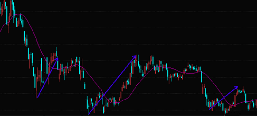
双均线策略

• 均线：对于每一个交易日，都可以计算出前N天的移动平均值，然后把这些移动平均值连起来，成为一条线，就叫做N日移动平均线。
• 移动平均线常用线有5天、10天、30天、60天、120天和240天的指标。 5天和10天的是短线操作的参照指标，称做日均线指标； 30天和60天的是中期均线指标，称做季均线指标； 120天、240天的是长期均线指标，称做年均线指标。
• 金叉：短期均线上穿长期均线
• 死叉：短期均线下穿长期均线

# 导入函数库
import jqdata

# 初始化函数，设定基准等等
def initialize(context):
    set_benchmark('000300.XSHG')
    set_option('use_real_price', True)
    set_order_cost(OrderCost(close_tax=0.001, open_commission=0.0003, close_commission=0.0003, min_commission=5), type='stock')
    
    g.security = ['601318.XSHG']
    g.p1 = 5
    g.p2 = 60
    
    
def handle_data(context, data):
    cash = context.portfolio.available_cash
    for stock in g.security:
        hist = attribute_history(stock, g.p2)
        ma60 = hist['close'].mean()
        ma5 = hist['close'][-5:].mean()
        if ma5 > ma60 and stock not in context.portfolio.positions:
            order_value(stock, cash/len(g.security))
        elif ma5 < ma60 and stock in context.portfolio.positions:
            order_target(stock, 0

因子选股策略

• 因子：
  • 标准 增长率，市值，ROE，……
• 选股策略：
  • 选取该因子最大（或最小）的N只股票持仓
• 多因子选股：如何同时考虑多个因子？

# 导入函数库
import jqdata

# 初始化函数，设定基准等等
def initialize(context):
    set_benchmark('000300.XSHG')
    set_option('use_real_price', True)
    set_order_cost(OrderCost(close_tax=0.001, open_commission=0.0003, close_commission=0.0003, min_commission=5), type='stock')
    g.N= 10
    g.days = 0
    
    #获取成分股
    
    
def handle_data(context, data):
    g.days+=1
    if g.days % 30 == 0:
        g.security = get_index_stocks('000300.XSHG')
        df = get_fundamentals(query(valuation).filter(valuation.code.in_(g.security)))
        df = df.sort(columns='market_cap')
        df = df.iloc[:g.N,:]
        tohold = df['code'].values
        
        for stock in context.portfolio.positions:
            if stock not in tohold:
                order_target(stock, 0)
                
        tobuy = [stock for stock in tohold if stock not in context.portfolio.positions]
        
        if len(tobuy)>0:
            cash = context.portfolio.available_cash
            cash_every_stock = cash / len(tobuy)
            for stock in tobuy:
                order_value(stock, cash_every_stock)

均值回归理论

import jqdata
import math
import numpy as np
import pandas as pd

def initialize(context):
    set_option('use_real_price', True)
    set_order_cost(OrderCost(close_tax=0.001, open_commission=0.0003, close_commission=0.0003, min_commission=5), type='stock')
    
    g.benchmark = '000300.XSHG'
    set_benchmark(g.benchmark)
    
    g.ma_days = 30
    g.stock_num = 10
    
    run_monthly(handle, 1)
    #run_monthly(handle, 11)
    
def handle(context):
    tohold = get_hold_list(context)
    for stock in context.portfolio.positions:
        if stock not in tohold:
            order_target_value(stock, 0)
    
    tobuy = [stock for stock in tohold if stock not in context.portfolio.positions]
    
    if len(tobuy)>0:
        cash = context.portfolio.available_cash
        cash_every_stock = cash / len(tobuy)
        
        for stock in tobuy:
            order_value(stock, cash_every_stock)

def get_hold_list(context):
    stock_pool = get_index_stocks(g.benchmark)
    stock_score = pd.Series(index=stock_pool)
    for stock in stock_pool:
        df = attribute_history(stock, g.ma_days, '1d', ['close'])
        ma = df.mean()[0]
        current_price = get_current_data()[stock].day_open
        ratio = (ma - current_price) / ma
        stock_score[stock] = ratio
    return stock_score.nlargest(g.stock_num).index.value

• 均值回归：“跌下去的迟早要涨上来”
• 均值回归的理论基于以下观测：价格的波动一般会以它的均线为中心。也就是说，当标的价格由于波动而偏离移动均线时，它将调整并重新归于均线。
• 偏离程度：(MA-P)/MA
• 策略：在每个调仓日进行（每月调一次仓）
  • 计算池内股票的N日移动均线；
  • 计算池内所有股票价格与均线的偏离度；
  • 选取偏离度最高的num_stocks支股票并进行调仓。

布林带策略

• 布林带/布林线/保利加通道（Bollinger Band）：由三条轨道线组成，其中上下两条线分别可以看成是价格的压力线和支撑线，在两条线之间是一条价格平均线。
• 计算公式：
  •  中间线=20日均线
  • up线=20日均线+N*SD(20日收盘价)
  • down线=20日均线-N*SD(20日收盘价)

import talib
#import numpy as np
#import pandas as pd

def initialize(context):
    set_option('use_real_price', True)
    set_order_cost(OrderCost(close_tax=0.001, open_commission=0.0003, close_commission=0.0003, min_commission=5), type='stock')
    set_benchmark('000300.XSHG')
    
    g.security = ['600036.XSHG']#,'601328.XSHG','600196.XSHG','600010.XSHG']
    g.N = 2
    
# 初始化此策略
def handle_data(context, data):
    cash = context.portfolio.cash / len(g.security)
    for stock in g.security:
        df = attribute_history(stock, 20)
        middle = df['close'].mean()
        upper = df['close'].mean() + g.N * df['close'].std()
        lower = df['close'].mean() - g.N * df['close'].std()
        
        current_price = get_current_data()[stock].day_open
        # 当价格突破阻力线upper时，且拥有的股票数量>=0时，卖出所有股票
        if current_price >= upper and stock in context.portfolio.positions:
            order_target(stock, 0)
        # 当价格跌破支撑线lower时, 且拥有的股票数量<=0时，则全仓买入
        elif current_price <= lower  and stock not in context.portfolio.positions:
            order_value(stock, cash)

PEG策略

• 彼得·林奇：任何一家公司股票如果定价合理的话，市盈率就会与收益增长率相等。
• 每股收益（EPS）
• 股价（P）
• 市盈率（PE）= P/EPS
• 收益增长率（G）= (EPSi – EPSi-1)/ EPSi-1
• PEG = PE / G / 100
• PEG越低，代表股价被低估的可能性越大，股价会涨的可能性越大。
• PEG是一个综合指标，既考察价值，又兼顾成长性。PEG估值法适合应用于成长型的公司。
• 注意：过滤掉市盈率或收益增长率为负的情况

def initialize(context):
    set_benchmark('000300.XSHG')
    set_option('use_real_price', True)
    set_order_cost(OrderCost(close_tax=0.001, open_commission=0.0003, close_commission=0.0003, min_commission=5), type='stock')
    
    g.security = get_index_stocks('000300.XSHG')
    g.days = 0
    g.N = 10
    
def handle_data(context, data):
    g.days+=1
    if g.days%30!=0:
        return
    df = get_fundamentals(query(valuation.code, valuation.pe_ratio, indicator.inc_net_profit_year_on_year).filter(valuation.code.in_(g.security)))
    df = df[(df['pe_ratio']>0)&(df['inc_net_profit_year_on_year']>0)]
    df['PEG'] = df['pe_ratio']/df['inc_net_profit_year_on_year']/100
    df = df.sort(columns='PEG')[:g.N]
    tohold = df['code'].values
    
    for stock in context.portfolio.positions:
        if stock not in tohold:
            order_target_value(stock, 0)
    
    tobuy = [stock for stock in tohold if stock not in context.portfolio.positions]
    
    if len(tobuy)>0:
        print('Buying')
        cash = context.portfolio.available_cash
        cash_every_stock = cash / len(tobuy)
        
        for stock in tobuy:
            order_value(stock, cash_every_stock)

羊驼交易法则

• 起始时随机买入N只股票，每天卖掉收益率最差的M只，再随机买入剩余股票池的M只。

import jqdata
import pandas as pd

def initialize(context):
    set_benchmark('000300.XSHG')
    set_option('use_real_price', True)
    set_order_cost(OrderCost(close_tax=0.001, open_commission=0.0003, close_commission=0.0003, min_commission=5), type='stock')
    
    g.security = get_index_stocks('000300.XSHG')
    g.period = 30
    g.N = 10
    g.change = 1
    g.init = True
    
    stocks = get_sorted_stocks(context, g.security)[:g.N]
    cash = context.portfolio.available_cash * 0.9 / len(stocks)
    for stock in stocks:
        order_value(stock, cash)
    run_monthly(handle, 2)
        
    
def get_sorted_stocks(context, stocks):
    df = history(g.period, field='close', security_list=stocks).T
    df['ret'] = (df.iloc[:,-1] - df.iloc[:,0]) / df.iloc[:,0]
    df = df.sort(columns='ret', ascending=False)
    return df.index.values
    
def handle(context):
    if g.init:
        g.init = False
        return
    stocks = get_sorted_stocks(context, context.portfolio.positions.keys())
    
    for stock in stocks[-g.change:]:
        order_target(stock, 0)
    
    stocks = get_sorted_stocks(context, g.security)
    
    for stock in stocks:
        if len(context.portfolio.positions) >= g.N:
            break
        if stock not in context.portfolio.positions:
            order_value(stock, context.portfolio.available_cash * 0.9)

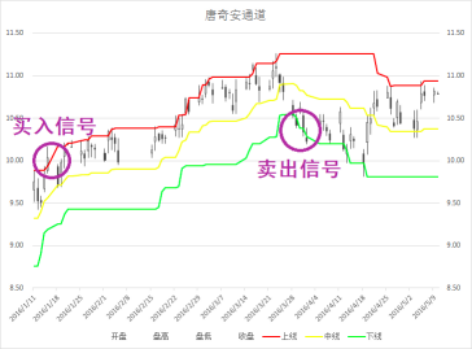
海龟交易法则

• 唐奇安通道：
  • 上线=Max（前N个交易日的最高价）
  • 下线=Min（前N个交易日的最低价）
  • 中线=（上线+下线）/2

 

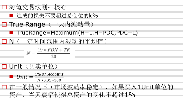
分钟回测

• 入市：若当前价格高于过去20日的最高价，则买入一个Unit
• 加仓：若股价在上一次买入（或加仓）的基础上上涨了0.5N，则加仓一个Unit
• 止盈：当股价跌破10日内最低价时（10日唐奇安通道下沿），清空头寸
• 止损：当价格比最后一次买入价格下跌2N时，则卖出全部头寸止损（损失不会超过2%）

 

import jqdata
import math
import numpy as np
import pandas as pd
from collections import deque

def initialize(context):
    
    set_option('use_real_price', True)
    set_order_cost(OrderCost(close_tax=0.001, open_commission=0.0003, close_commission=0.0003, min_commission=5), type='stock')

    g.security = '000060.XSHE'
    set_benchmark(g.security)
    g.in_day = 20
    g.out_day = 10
    g.today_units = 0
    g.current_units = 0
    g.N=deque(maxlen=19)
    g.current_N = 0
    g.last_buy_price = 0
    
    price = attribute_history(g.security, g.N.maxlen*2+1, '1d', ('high', 'low', 'close'))
    
    for i in range(g.N.maxlen+1, g.N.maxlen*2+1):
        li = []
        for j in range(i-19,i+1):
            a = price['high'][j]-price['low'][j]
            b = abs(price['high'][j]-price['close'][j-1])
            c = abs(price['low'][j]-price['close'][j-1])
            li.append(max(a,b,c))
        current_N = np.array(li).mean()
        g.N.append(current_N)
        
    
def before_trading_start(context):
    g.current_N = cal_N()
    g.today_units = 0

    
def handle_data(context, data):
    dt = context.current_dt
    current_price = data[g.security].price #上一分钟价格
    value = context.portfolio.total_value
    cash = context.portfolio.available_cash
    
    unit = math.floor(value * 0.01 / g.current_N)
    
        
    if g.current_units == 0:
        buy(current_price, cash, unit)
    else:
        if stop_loss(current_price):
            return
        if sell(current_price):
            return
        addin(current_price, cash, unit)
    
def cal_N():
    # if len(g.N) < g.N.maxlen:
    #     price = attribute_history(g.security, g.N.maxlen+2, '1d', ('high', 'low', 'close'))
    #     li = []
    #     for i in range(1, g.N.maxlen+2):
    #         a = price['high'][i]-price['low'][i]
    #         b = abs(price['high'][i]-price['close'][i-1])
    #         c = abs(price['low'][i]-price['close'][i-1])
    #         li.append(max(a,b,c))
    #     current_N = np.array(li).mean()
    # else:
    price = attribute_history(g.security, 2, '1d', ('high', 'low', 'close'))
    a = price['high'][1]-price['low'][1]
    b = abs(price['high'][1]-price['close'][0])
    c = abs(price['low'][1]-price['close'][0])
    current_N = (max(a,b,c) + np.array(g.N).sum())/(g.N.maxlen+1)
    g.N.append(current_N)
    return current_N
    
def buy(current_price, cash, unit):
    price = attribute_history(g.security, g.in_day, '1d', ('high',))
    if current_price > max(price['high']):
        shares = cash / current_price
        if shares >= unit:
            print("buying %d" % unit)
            o = order(g.security, unit)
            g.last_buy_price = o.price
            g.current_units += 1
            g.today_units += 1
            return True
    return False
            

def addin(current_price, cash, unit):
    if current_price >= g.last_buy_price + 0.5 * g.current_N:
        shares = cash / current_price
        if shares >= unit:
            print("adding %d" % unit)
            o = order(g.security, unit)
            g.last_buy_price = o.price
            g.current_units += 1
            g.today_units += 1
            return True
    return False
            
def sell(current_price):
    price = attribute_history(g.security, g.out_day, '1d', ('low',))
    if current_price < min(price['low']):
        print("selling")
        order_target(g.security, 0)
        g.current_units = g.today_units
        return True
    return False
        
def stop_loss(current_price):
    if current_price < g.last_buy_price - 2 * g.current_N:
        print("stop loss")
        order_target(g.security, 0)
        g.current_units = g.today_units
        return True
    return False

 

鳄鱼法则交易系统

https://www.joinquant.com/post/595?tag=new

# 导入函数库
import jqdata
import numpy as np

# 初始化函数，设定基准等等
def initialize(context):
    set_option('use_real_price', True)
    set_order_cost(OrderCost(close_tax=0.001, open_commission=0.0003, close_commission=0.0003, min_commission=5), type='stock')
    set_benchmark('000300.XSHG')
    
    g.up_price = {} #向上碎形最高价
    g.low_price = {} #向下碎形最低价
    g.up_fractal_exists = {} #判断有效向上碎形
    g.down_fractal_exists = {} #判断有效向下碎形
    g.AO_index = {} #存放连续的AO指标数据
    g.cal_AC_index = {} #计算AC指标中转存储
    g.AC_index = {} #存放连续的AC指标数据
    g.amount = {} #满仓仓位
    g.stock = get_index_stocks('000300.XSHG')
    g.buy_stock = []
    g.month = context.current_dt.month
    run_monthly(select_universe,1,'open')
    
#重置全局变量
def reset_global():
    g.up_price = {} #向上碎形最高价
    g.low_price = {} #向下碎形最低价
    g.up_fractal_exists = {} #判断有效向上碎形
    g.down_fractal_exists = {} #判断有效向下碎形
    g.AO_index = {} #存放连续的AO指标数据
    g.cal_AC_index = {} #计算AC指标中转存储
    g.AC_index = {} #存放连续的AC指标数据
    g.amount = {} #满仓仓位
    g.buy_stock = []

def initial_stock_global(stock):
    g.up_price[stock] = 0
    g.low_price[stock] = 0
    g.up_fractal_exists[stock] = False
    g.down_fractal_exists[stock] = False #判断有效向下碎形
    g.AO_index[stock] = [0] #存放连续的AO指标数据
    g.cal_AC_index[stock] = [0]  #计算AC指标中转存储
    g.AC_index[stock] = [0] #存放连续的AC指标数据
    g.amount[stock] = 0 #满仓仓位

#轮换选股后清空持仓
def reset_position(context):
    for stock in g.buy_stock:
        order_target(stock,0)
        log.info("sell %s for reset position"%stock)

#选股
def select_universe(context):
    #每三个月操作一次
    month = context.current_dt.month
    if month%6 != g.month%6:
        return
    #清空全局变量
    reset_position(context)
    reset_global()
    hist = history(30,'1d','close',g.stock,df = False)
    for stock in g.stock:
        if is_sleeping_alligator(stock,hist,20):
            g.buy_stock.append(stock)
            #初始化该股票全局变量
            initial_stock_global(stock)
    print g.buy_stock
    return None
    
#睡着的鳄鱼
def is_sleeping_alligator(stock,hist,nday):
    for i in range(nday):
        if is_struggle(stock,hist,i) == False:
            return False
    return True

#均线纠缠，BRG三线非常接近
def is_struggle(stock,hist,delta):
    blue_line = hist[stock][-21-delta:-8-delta].mean()
    red_line = hist[stock][-13-delta:-5-delta].mean()
    green_line = hist[stock][-8-delta:-3-delta].mean()
    if abs(blue_line/red_line-1)<0.02 and abs(red_line/green_line-1)<0.02:
        return True
    else:
        return False
        
#判断 向上 或 向下 碎形
def is_fractal(stock,direction):
    hist = attribute_history(stock, 5, fields=[direction])
    if direction == 'high':
        if np.all(hist.iloc[:2] < hist.iloc[2]) and np.all(hist.iloc[3:] < hist.iloc[2]):
            g.up_price[stock] = hist.iloc[2].values
            return True
    elif direction == 'low':
        if np.all(hist.iloc[:2] > hist.iloc[2]) and np.all(hist.iloc[3:] > hist.iloc[2]):
            g.low_price[stock] = hist.iloc[2].values
            return True
    return False
    
#通过比较碎形与红线位置，判断碎形是否有效
def is_effective_fractal(stock, direction):
    if is_fractal(stock,direction):
        hist = attribute_history(stock, 11)
        red_line = hist['close'][:-3].mean()
        close_price = hist['close'][-1]
        if direction == 'high':
            if close_price > red_line:
                g.up_fractal_exists[stock] = True
            else:
                g.up_fractal_exists[stock] = False
        elif direction == 'low':
            if close_price < red_line:
                g.down_fractal_exists[stock] = True
            else:
                g.down_fractal_exists[stock] = False
    

#N日内最高价格的N日线
def nday_high_point(stock,n):
    hist = history(2*n,'1d','high',[stock],df = False)[stock]
    high_point = []
    for i in range(n):
        high_point.append(max(hist[-5-i:-1-i]))
    return np.array(high_point).mean()

#N日内最低价格的N日线
def nday_low_point(stock,n):
    hist = history(2*n,'1d','low',[stock],df = False)[stock]
    low_point = []
    for i in range(n):
        low_point.append(max(hist[-5-i:-1-i]))
    return np.array(low_point).mean()

#AO=5日内（最高-最低）/2的5日移动平均-34日内（最高-最低）/2的34日移动平均
def AO_index(stock):
    g.AO_index[stock].append(nday_high_point(stock,5)/2 + nday_low_point(stock,5)/2\
                      - nday_high_point(stock,34)/2 - nday_low_point(stock,34)/2)
    return None

#AO-AO的5日平均值的5日平均
def AC_index(stock):
    AO_index(stock)
    if len(g.AO_index[stock]) >= 5:
        g.cal_AC_index[stock].append(g.AO_index[stock][-1] - np.array(g.AO_index[stock][-5:]).mean())
        if len(g.cal_AC_index[stock]) >=5:
            g.AC_index[stock].append(np.array(g.cal_AC_index[stock][-5:]).mean())

#判断序列n日上行
def is_up_going(alist,n):
    if len(alist) < n:
        return False
    for i in range(n-1):
        if alist[-(1+i)] <= alist[-(2+i)]:
            return False
    return True

#判断序列n日下行
def is_down_going(alist,n):
    if len(alist) < n:
        return False
    for i in range(n-1):
        if alist[-(1+i)] >= alist[-(2+i)]:
            return False
    return True

#碎形被突破
def active_fractal(stock,direction):
    close_price = history(1,'1d','close',[stock],df=False)[stock][0]
    if direction == 'up' and close_price > g.up_price[stock]:
        return True
    elif direction == 'down' and close_price < g.low_price[stock]:
        return True
    return False

#进场，初始仓位
def set_initial_position(stock,context):
    close_price = history(1,'1d','close',[stock],df=False)[stock][0]
    g.amount[stock] = context.portfolio.cash/close_price/len(g.buy_stock)*3
    order(stock, g.amount[stock])
    log.info("buying %s 股数为 %s"%(stock,g.amount[stock]))
    g.down_fractal_exists[stock] = False

#卖出
def sell_all_stock(stock,context):
    order_target(stock,0)
    log.info("selling %s"%stock)
    g.up_fractal_exists[stock] = False

#加仓
def adjust_position(stock,context,position):
    order(stock,g.amount[stock]*position)
    log.info("adjust position buying %s 股数为 %s"%(stock,g.amount[stock]*position))

# 计算股票前n日收益率
def security_return(days,security_code):
    hist1 = attribute_history(security_code, days + 1, '1d', 'close',df=False)
    security_returns = (hist1['close'][-1]-hist1['close'][0])/hist1['close'][0]
    return security_returns

# 止损，根据前n日收益率
def conduct_nday_stoploss(context,security_code,days,bench):
    if  security_return(days,security_code)<= bench:
        for stock in g.buy_stock:
            order_target_value(stock,0)
            log.info("Sell %s for stoploss" %stock)
        return True
    else:
        return False

# 计算股票累计收益率（从建仓至今）
def security_accumulate_return(context,data,stock):
    current_price = data[stock].price
    cost = context.portfolio.positions[stock].avg_cost
    if cost != 0:
        return (current_price-cost)/cost
    else:
        return None

# 个股止损，根据累计收益
def conduct_accumulate_stoploss(context,data,stock,bench):
    if security_accumulate_return(context,data,stock) != None\
    and security_accumulate_return(context,data,stock) < bench:
        order_target_value(stock,0)
        log.info("Sell %s for stoploss" %stock)
        return True
    else:
        return False

# 个股止盈，根据累计收益
def conduct_accumulate_stopwin(context,data,stock,bench):
    if security_accumulate_return(context,data,stock) != None\
    and security_accumulate_return(context,data,stock) > bench:
        order_target_value(stock,0)
        log.info("Sell %s for stopwin" %stock)
        return True
    else:
        return False

def handle_data(context,data):
    #大盘止损
    if conduct_nday_stoploss(context,'000300.XSHG',3,-0.03):
        return
    for stock in g.buy_stock:
        #个股止损
        if conduct_accumulate_stopwin(context,data,stock,0.3)\
        or conduct_accumulate_stoploss(context,data,stock,-0.1):
            return
        #计算AO，AC指标
        AC_index(stock)
        #空仓时，寻找机会入场
        if context.portfolio.positions[stock].amount == 0:
            #计算向上碎形
            is_effective_fractal(stock,'high')
            #有效向上碎形存在，并被突破，买入
            if g.up_fractal_exists and active_fractal(stock,'up'):
                close_price = history(5, '1d', 'close', [stock],df = False)
                if is_up_going(g.AO_index[stock],5)\
                and is_up_going(g.AC_index[stock],3)\
                and is_up_going(close_price[stock],2):
                    set_initial_position(stock,context)
        #有持仓时，加仓或离场
        else:
            #计算向下碎形
            is_effective_fractal(stock,'low')
            #出场条件1：有效向下碎形存在，并被突破，卖出
            if g.down_fractal_exists and active_fractal(stock,'down'):
                sell_all_stock(stock,context)
                return