

统计学习方法——svm
效率???
SMO参考链接:
http://svmlight.joachims.org/
https://www.csie.ntu.edu.tw/~cjlin/libsvm/#download
包含的内容如下:
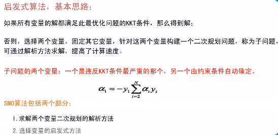
启发式搜索算法 优化算法参考链接:
https://blog.csdn.net/u011835903/category_10226833_2.html 智能优化算法网址
https://blog.csdn.net/u011835903/article/details/110523352 基于麻雀搜索算法优化的SVM数据分类预测
https://blog.csdn.net/u011835903/article/details/107716390智能优化算法:灰狼优化算法原理——附代码
https://blog.csdn.net/u011835903/article/details/107535864智能优化算法:海鸥优化算法原理——附代码
https://blog.csdn.net/u011835903/article/details/107559167智能优化算法:鲸鱼优化算法原理——附代码
#!/usr/bin/env python3
# -*- coding: utf-8 -*-
' 统计学习方法 —— 支持向量机 (support vector machines——SVM) '
'svm 对应的凸二次规划问题的最优化算法有很多,以下是其中之一实现:' \
' 序列最小最优化算法(sequential minimal optimization——SMO) '
' 初始参数输入: ' \
' 1. 惩罚参数C (C > 0) :C值大时对误差分类的惩罚增大, C值小时对误差分类的惩罚减小,在间隔尽量大(欠拟合)和 误分类点数尽量少(过拟合) 之间做调和' \
' 2. 核函数kernelFunc : 常用核函数 线性svm; "polynomial": 多项式; "gaussian": 高斯;' \
__author__ = 'qfr'
import matplotlib
import matplotlib.pyplot as plt
import numpy as np
from numpy import *;#导入numpy的库函数
import sys
import random
import copy
import datetime
# SMO算法实现
class SVM_Smo(object):
def __init__(self, c = 100, kfunc = "polynomial", sigma = 1.0, p = 1.0):
# 初始参数设置
self.__c = c # 惩罚参数
self.__sigma = sigma # 高斯核函数 标准差参数
self.__p = p # 多项式核函数的幂次方
if kfunc == "polynomial":
self.__kernelFunc = self.__CalcKPolynomial
else:
self.__kernelFunc = self.__CalcKGaussian
self.__b = 0.0
self.__pointId = []
# 多项式核函数计算
def __CalcKPolynomial(self, x1, x2):
sum = 0;
for i in range(x1.size):
sum = sum + x1[i] * x2[i]
return (sum + 1)**self.__p
# 高斯核函数计算
def __CalcKGaussian(self, x1, x2):
sum = 0;
for i in range(x1.size):
tem = (x1[i] - x2[i]) ** 2
sum = sum + tem
tem = -1.0 * sum / 2.0 / (self.__sigma ** 2)
return np.exp(tem)
# 计算g(xi)
def __CalcGxi(self, xi):
sum = 0.0
for i in range(self.__a.size):
tem = self.__a[i] * self.__y[i] * self.__kernelFunc(xi, self.__x[i])
sum = sum + tem
return sum + self.__b
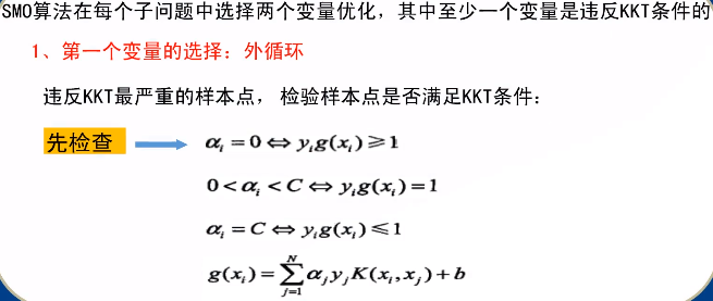
# 选择第一个变量
def __SelectA1(self, g):
# 先遍历 在间隔边界上的支持向量点 0 < a[i] < C
for i in range(self.__a.size):
if self.__a[i] > 0 and self.__a[i] < self.__c:
if not math.isclose(self.__y[i] * g[i], 1.0, abs_tol=1e-08): # 违反KKT条件
return i
# 其次, 遍历 大于间隔边界的样本 a[i] == 0
for i in range(self.__a.size):
if math.isclose(self.__a[i], 0.0, abs_tol=1e-08):
if self.__y[i] * g[i] < 1.0: # 违反KKT条件
return i
# 最后, 遍历间隔边界以里的边界点 a[i] == C (可能在间隔边界和分离超平面之前,可能在分离超平面另一侧,即误分类)
for i in range(self.__a.size):
if math.isclose(self.__a[i], self.__c, abs_tol=1e-08):
if self.__y[i] * g[i] > 1.0: # 违反KKT条件
return i
return -1
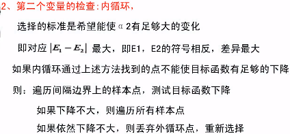
# 选择第二个变量
def __SelectA2(self, e, idx1):
# 1 选择|E1-E2|最大的 a2
max = 0.0
idx2 = -1
for i in range(e.size):
if idx1 == i:
continue
newA1, newA2 = self.__UpdateA12(e, idx1, i)
tem = abs(newA2) # abs(e[idx1] - e[i])
if tem > max:
max = tem
idx2 = i
# 2 如果选择的a2不能使目标函数有足够的下降,采用启发式规则继续选择a2, 直到目标函数有足够的下降
# 2.1 先遍历间隔边界上的支持向量点
# 2.2 其次遍历整个数据集
# 2.3 最后放弃第一个a1, 通过外层循环寻求另一个a1
return idx2
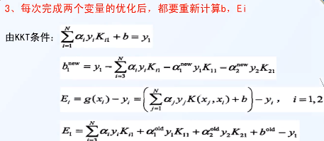
def __UpdateEi(self, g, e):
for i in range(self.__a.size):
g[i] = self.__CalcGxi(self.__x[i])
e[i] = g[i] - self.__y[i]
def __UpdateA12(self, e, idx1, idx2):
# 求上下边界
l = zeros(2)
h = zeros(2)
if math.isclose(self.__y[idx1], self.__y[idx2], abs_tol=1e-08):
l[0] = 0
l[1] = self.__a[idx2] + self.__a[idx1] - self.__c
h[0] = self.__c
h[1] = self.__a[idx2] + self.__a[idx1]
else:
l[0] = 0
l[1] = self.__a[idx2] - self.__a[idx1]
h[0] = self.__c
h[1] = self.__c + self.__a[idx2] - self.__a[idx1]
hMin = h.min()
lMax = l.max()
# 更新a2
k11 = self.__kernelFunc(self.__x[idx1], self.__x[idx1])
k22= self.__kernelFunc(self.__x[idx2], self.__x[idx2])
k12 = self.__kernelFunc(self.__x[idx1], self.__x[idx2])
n = k11 + k22 - 2 * k12
newA2 = self.__a[idx2] + self.__y[idx2] * (e[idx1] - e[idx2]) / n
# 边界限制
if newA2 > hMin:
newA2 = hMin
if newA2 < lMax:
newA2 = lMax
# 更新a1
newA1 = self.__a[idx1] + self.__y[idx1] * self.__y[idx2] * (self.__a[idx2] - newA2)
return newA1, newA2
def __UpdateB(self, e, newA1, newA2, idx1, idx2):
k11 = self.__kernelFunc(self.__x[idx1], self.__x[idx1])
k22 = self.__kernelFunc(self.__x[idx2], self.__x[idx2])
k12 = self.__kernelFunc(self.__x[idx1], self.__x[idx2])
b1_new = self.__b - e[idx1] - self.__y[idx1] * k11 * (newA1 - self.__a[idx1]) - \
self.__y[idx2] * k12 * (newA2 - self.__a[idx2])
b2_new = self.__b - e[idx2] - self.__y[idx2] * k22 * (newA2 - self.__a[idx2]) - \
self.__y[idx1] * k12 * (newA1 - self.__a[idx1])
if newA1 > 0 and newA1 < self.__c:
tem = b1_new
elif newA2 > 0 and newA2 < self.__c:
tem = b2_new
else:
tem = (b1_new + b2_new) / 2.0
#print("b", tem - self.__b)
self.__b = tem
# smo迭代停止判断
def __IsIterationStop(self, g):
sum = 0.0
for i in range(self.__a.size):
sum = sum + self.__a[i] * self.__y[i]
tem = self.__y[i] * g[i]
if self.__a[i] > 0 and self.__a[i] < self.__c:
if not math.isclose(tem, 1.0, abs_tol=1e-08):
#print("边界点不满足")
return False
elif math.isclose(self.__a[i], 0.0, abs_tol=1e-08):
if tem < 1.0:
#print("正确分类点不满足")
return False
elif math.isclose(self.__a[i], self.__c, abs_tol=1e-08):
if tem > 1.0:
#print("误分类点不满足")
return False
else:
print("异常情况不满足")
return False
if math.isclose(sum, 0.0, abs_tol=1e-08):
print("训练完成 done!!!")
return True
return False
# smo迭代优化
def __SmoIteration(self):
# 中间定义
g = np.zeros(self.__y.size)
e = np.zeros(self.__y.size)
self.__UpdateEi(g, e)
# 循环更新
while True:
# 选择a1 a2
idx1 = self.__SelectA1(g)
if idx1 < 0:
break
idx2 = self.__SelectA2(e, idx1)
if idx2 < 0:
continue
# 更新a, b
newA1, newA2 = self.__UpdateA12(e, idx1, idx2)
#print("idx1:", idx1, "a:", newA1 - self.__a[idx1])
#print("idx2:", idx2, "a:", newA2 - self.__a[idx2])
self.__UpdateB(e, newA1, newA2, idx1, idx2)
self.__a[idx1] = newA1
self.__a[idx2] = newA2
# 重新计算中间变量
self.__UpdateEi(g, e)
# 判断是否停止
if self.__IsIterationStop(g):
break
# 数据输入,训练入口
def Smo(self, dataT, dataY):
# 初始内部参数保存
self.__x = dataT
self.__y = dataY
self.__a = np.zeros(dataY.size)
# 训练模型
self.__SmoIteration()
# 存储支持向量点Id
for i in range(self.__a.size):
if self.__a[i] > 0 and self.__a[i] < self.__c:
self.__pointId.append(i)
# 计算并返回支撑向量点
def GetSvmPoint(self):
svmX = []
svmY = []
for i in self.__pointId:
svmX.append(self.__x[i][0])
svmY.append(self.__x[i][1])
return svmX, svmY
# 计算并返回分离曲面
def GetSvmSurface(self):
pass
# 预测新的数据分类
def predict(self, x):
y = []
for i in x:
tem = self.__CalcGxi(i)
if tem >= 0:
y.append(1)
else:
y.append(-1)
return np.array(y)
# 计算样本点到计算超平面的函数距离
def decision_function(self, x):
y = []
for i in x:
tem = self.__CalcGxi(i)
if tem >= 0:
y.append(tem)
else:
y.append(-1.0 * tem)
return np.array(y)
def plot_dataset(X, y, axes):
plt.plot( X[:,0][y==-1], X[:,1][y==-1], "bs" )
plt.plot( X[:,0][y==1], X[:,1][y==1], "g^" )
plt.axis( axes )
plt.grid( True, which="both" )
plt.xlabel(r"$x_l$")
plt.ylabel(r"$x_2$")
# contour函数是画出轮廓,需要给出X和Y的网格,以及对应的Z,它会画出Z的边界(相当于边缘检测及可视化)
def plot_predict(s, axes):
x0s = np.linspace(axes[0], axes[1], 200)
x1s = np.linspace(axes[2], axes[3], 200)
x0, x1 = np.meshgrid(x0s, x1s)
X = np.c_[x0.ravel(), x1.ravel()]
y_pred = s.predict(X).reshape(x0.shape)
y_decision = s.decision_function(X).reshape(x0.shape)
plt.contour(x0, x1, y_pred, cmap=plt.cm.winter, alpha=0.8)
C = plt.contour( x0, x1, y_decision, cmap=plt.cm.winter, alpha=0.2 )
plt.clabel(C, inline=True, fontsize=10)
if __name__=='__main__':
start = datetime.datetime.now()
fig1 = plt.figure()
# 生成原始数据
sigma = 3.0
# 正类设置
numP = 10
xp0 = 30
xp1 = 50
# 负类设置
numN = 10
xn0 = 20
xn1 = 58
noise = sigma * np.random.randn(numP, 1)
xp_1 = noise + xp0
noise = sigma * np.random.randn(numP, 1)
xp_2 = noise + xp1
yp = np.ones(numP)
sigma = 1
noise = sigma * np.random.randn(numN, 1)
xn_1 = noise + xn0
noise = sigma * np.random.randn(numN, 1)
xn_2 = noise + xn1
yn = -1 * np.ones(numN)
# 组成训练数据集
Tp = np.insert(xp_1, [1], xp_2, axis=1)
Tn = np.insert(xn_1, [1], xn_2, axis=1)
T = np.vstack((Tp, Tn)) # 训练数据集
Y = np.hstack((yp, yn)) # 标记结果
# 对结果进行乱序
for i in reversed(range(1, len(Y))):
# pick an element in x[:i+1] with which to exchange x[i]
j = np.random.randint(0, i + 1, 1)[0]
Y[i], Y[j] = Y[j], Y[i]
cc = copy.deepcopy(T[i])
T[i] = copy.deepcopy(T[j])
T[j] = copy.deepcopy(cc)
end = datetime.datetime.now()
start = end
print("数据准备完成:", end - start)
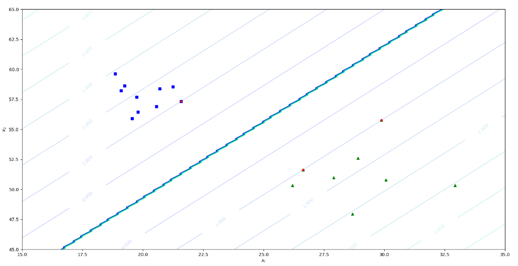
plot_dataset(T, Y, [15, 35, 45, 65]);
s = SVM_Smo(c = 1)
s.Smo(T, Y)
end = datetime.datetime.now()
print("数据训练done:", end - start)
# 绘制分割线相关信息
sx, sy = s.GetSvmPoint()
plt.plot(sx, sy, 'r*')
plot_predict(s, [15, 35, 45, 65])
plt.show()
训练结果如下,示例:
记录每天生活的点点滴滴,呵呵呵呵呵呵

 浙公网安备 33010602011771号