Keras下的文本情感分析简介。与MLP,RNN,LSTM模型下的文本情感测试


  1 # coding: utf-8
  2
  3 # In[1]:
  4
  5
  6 import urllib.request
  7 import os
  8 import tarfile
  9
 10
 11 # In[2]:
 12
 13
 14 url="http://ai.stanford.edu/~amaas/data/sentiment/aclImdb_v1.tar.gz"
 15 filepath="example/data/aclImdb_v1.tar.gz"
 16 if not os.path.isfile(filepath):
 17     result=urllib.request.urlretrieve(url,filepath)
 18     print('downloaded:',result)
 19 if not os.path.exists("example/data/aclImdb_v1/aclImdb"):
 20     tfile = tarfile.open("data/aclImdb_v1.tar.gz", 'r:gz')
 21     result=tfile.extractall('data/')
 22
 23
 24 # In[3]:
 25
 26
 27 from keras.datasets import imdb
 28 from keras.preprocessing import sequence
 29 from keras.preprocessing.text import Tokenizer
 30
 31
 32 # In[4]:
 33
 34
 35 import re
 36 def rm_tags(text):
 37     re_tag = re.compile(r'<[^>]+>')
 38     return re_tag.sub('', text)
 39
 40
 41 # In[5]:
 42
 43
 44 import os
 45 def read_files(filetype):
 46     path = "example/data/aclImdb_v1/aclImdb/"
 47     file_list=[]
 48
 49     positive_path=path + filetype+"/pos/"
 50     for f in os.listdir(positive_path):
 51         file_list+=[positive_path+f]
 52
 53     negative_path=path + filetype+"/neg/"
 54     for f in os.listdir(negative_path):
 55         file_list+=[negative_path+f]
 56
 57     print('read',filetype, 'files:',len(file_list))
 58     all_labels = ([1] * 12500 + [0] * 12500)
 59
 60     all_texts  = []
 61     for fi in file_list:
 62         with open(fi,encoding='utf8') as file_input:
 63             all_texts += [rm_tags(" ".join(file_input.readlines()))]
 64
 65     return all_labels,all_texts
 66
 67
 68 # In[6]:
 69
 70
 71 y_train,train_text=read_files("train")
 72
 73
 74 # In[7]:
 75
 76
 77 y_test,test_text=read_files("test")
 78
 79
 80 # In[8]:
 81
 82
 83 train_text[0]
 84
 85
 86 # In[9]:
 87
 88
 89 y_train[0]
 90
 91
 92 # In[10]:
 93
 94
 95 train_text[12500]
 96
 97
 98 # In[11]:
 99
100
101 y_train[12500]
102
103
104 # In[12]:
105
106
107 token = Tokenizer(num_words=2000)
108 token.fit_on_texts(train_text)
109
110
111 # In[13]:
112
113
114 print(token.document_count)
115 print(token.word_index)
116
117
118 # In[14]:
119
120
121 x_train_seq = token.texts_to_sequences(train_text)
122 x_test_seq  = token.texts_to_sequences(test_text)
123
124
125 # In[15]:
126
127
128 print(x_train_seq[0])
129
130
131 # In[16]:
132
133
134 x_train = sequence.pad_sequences(x_train_seq, maxlen=100)
135 x_test  = sequence.pad_sequences(x_test_seq,  maxlen=100)
136
137
138 # In[17]:
139
140
141 x_train[0]
142
143
144 # In[18]:
145
146
147 from keras.models import Sequential
148 from keras.layers.core import Dense, Dropout, Activation,Flatten
149 from keras.layers.embeddings import Embedding
150 model = Sequential()
151 model.add(Embedding(output_dim=32,
152                     input_dim=2000,
153                     input_length=100))
154 model.add(Dropout(0.2))
155 model.add(Flatten())
156 model.add(Dense(units=256,
157                 activation='relu' ))
158 model.add(Dropout(0.2))
159 model.add(Dense(units=1,
160                 activation='sigmoid' ))
161 model.summary()
162
163
164 # In[19]:
165
166
167 model.compile(loss='binary_crossentropy',
168               optimizer='adam',
169               metrics=['accuracy'])
170 train_history =model.fit(x_train, y_train,batch_size=100,
171                          epochs=10,verbose=2,
172                          validation_split=0.2)
173
174
175 # In[20]:
176
177
178 get_ipython().magic('pylab inline')
179 import matplotlib.pyplot as plt
180 def show_train_history(train_history,train,validation):
181     plt.plot(train_history.history[train])
182     plt.plot(train_history.history[validation])
183     plt.title('Train History')
184     plt.ylabel(train)
185     plt.xlabel('Epoch')
186     plt.legend(['train', 'validation'], loc='upper left')
187     plt.show()
188
189
190 # In[21]:
191
192
193 show_train_history(train_history,'acc','val_acc')
194 show_train_history(train_history,'loss','val_loss')
195
196
197 # In[22]:
198
199
200 scores = model.evaluate(x_test, y_test, verbose=1)
201 scores[1]
202
203
204 # In[23]:
205
206
207 probility=model.predict(x_test)
208
209
210 # In[24]:
211
212
213 probility[:10]
214
215
216 # In[25]:
217
218
219 probility[12500:12510]
220
221
222 # In[26]:
223
224
225 predict=model.predict_classes(x_test)
226
227
228 # In[27]:
229
230
231 predict_classes=predict.reshape(-1)
232
233
234 # In[28]:
235
236
237 SentimentDict={1:'正面的',0:'负面的'}
238 def display_test_Sentiment(i):
239     print(test_text[i])
240     print('标签label:',SentimentDict[y_test[i]],
241           '预测结果:',SentimentDict[predict_classes[i]])
242
243
244 # In[29]:
245
246
247 display_test_Sentiment(2)
248
249
250 # In[30]:
251
252
253 display_test_Sentiment(12505)
254
255
256 # In[31]:
257
258
259 from keras.models import Sequential
260 from keras.layers.core import Dense, Dropout, Activation
261 from keras.layers.embeddings import Embedding
262 from keras.layers.recurrent import SimpleRNN
263 model = Sequential()
264 model.add(Embedding(output_dim=32,
265                     input_dim=2000,
266                     input_length=100))
267 model.add(Dropout(0.35))
268 model.add(SimpleRNN(units=16))
269 model.add(Dense(units=256,activation='relu' ))
270 model.add(Dropout(0.35))
271 model.add(Dense(units=1,activation='sigmoid' ))
272 model.summary()
273
274
275 # In[32]:
276
277
278 model.compile(loss='binary_crossentropy',
279               optimizer='adam',
280               metrics=['accuracy'])
281 train_history =model.fit(x_train, y_train,batch_size=100,
282                          epochs=10,verbose=2,
283                          validation_split=0.2)
284
285
286 # In[33]:
287
288
289 scores = model.evaluate(x_test, y_test, verbose=1)
290 scores[1]
291
292
293 # In[34]:
294
295
296 from keras.models import Sequential
297 from keras.layers.core import Dense, Dropout, Activation,Flatten
298 from keras.layers.embeddings import Embedding
299 from keras.layers.recurrent import LSTM
300 model = Sequential()
301 model.add(Embedding(output_dim=32,
302                     input_dim=2000,
303                     input_length=100))
304 model.add(Dropout(0.2))
305 model.add(LSTM(32))
306 model.add(Dense(units=256,
307                 activation='relu' ))
308 model.add(Dropout(0.2))
309 model.add(Dense(units=1,
310                 activation='sigmoid' ))
311 model.summary()
312
313
314 # In[35]:
315
316
317 model.compile(loss='binary_crossentropy',
318               #optimizer='rmsprop',
319               optimizer='adam',
320               metrics=['accuracy'])
321 train_history =model.fit(x_train, y_train,batch_size=100,
322                          epochs=10,verbose=2,
323                          validation_split=0.2)
324
325
326 # In[36]:
327
328
329 show_train_history(train_history,'acc','val_acc')
330 show_train_history(train_history,'loss','val_loss')
331 scores = model.evaluate(x_test, y_test, verbose=1)
332 scores[1]
333
334
335 # In[ ]:
文本来源于IMDb网络电影数据集。下载,放到合适的路径下,然后,开始。
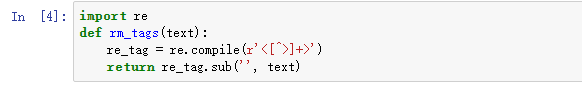
过滤掉HTML标签。因为数据集中有相关标签。:
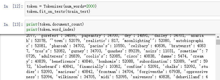
之后读取所有数据和目标标签,然后建立字典:
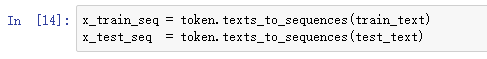
将文本转化为数字串:
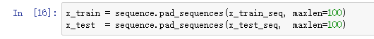
格式化数字串长度为100
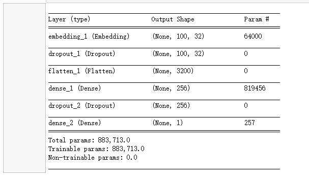
建立MLP模型,其中嵌入层将每个长度为100的数字串转为100个32维的向量,将文字映射成多维的几何空间向量,让每一个文字有上下的关联性。
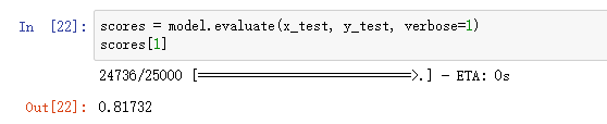
编译,训练,绘图,评估后的准确率:
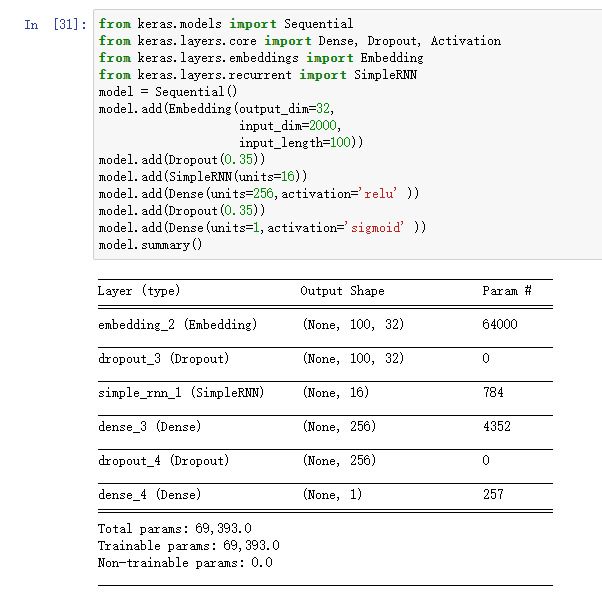
建立RNN模型,有关RNN模型的介绍:https://www.cnblogs.com/bai2018/p/10466418.html
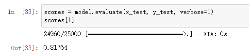
测试评估:
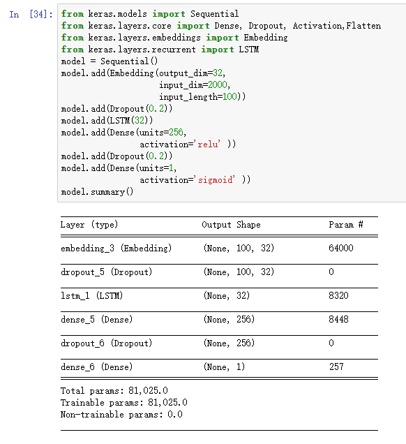
建立LSTM模型,相关介绍:https://www.cnblogs.com/bai2018/p/10466497.html
准确率:

Le vent se lève! . . . il faut tenter de vivre!
Le vent se lève! . . . il faut tenter de vivre!

 浙公网安备 33010602011771号