Cloth Simulation with Root Finding and Optimization

目录

• 0 前言
• 1 Implicit Method
  • 1.1 Root-finding
  • 1.2 Optimization
  • 1.3 Insight
• 2 Newton-Raphson Method
• 3 Mass-Spring System
  • 3.1 Matrix calculus
  • 3.2 A Spring with Two Ends
• 4 Explaination of Init Code with 3D Image
  • 4.1 Initialize
  • 4.2 Index
  • 4.3 Edge
  • 4.4 Sort Edge
• 5 Update
• 6 Get_Gradient
  • 6.1 first derivative
  • 6.2 second derivative
• 7 Collision_Handling

0 前言

声明：此篇博客仅用于个人学习记录之用，并非是分享代码。Hornor the Code

我只能说，衣料模拟的技术深度比3D刚体模拟的技术深太多了。这次的实验参考了许多资料，包括

• 《University of Tennessee MES301 Fall, 2023》
• 《Root finding and optimization: Scientific Computing for Physicists 2017》
• 《Physics-based animation lecture 5: OH NO! It's More Finite Elements》 这个老师讲课用一个小猫，特逗
• 当然主要还是 Games103王华民老师的《Intro to Physics-Based Animation!》

里面用到的一些技术，在有限元里也有应用。

另外还有不基于物理的衣料模拟 《Position Based Dynamics》, 这个是05年左右开始出现的技术。详细的内容可以看PBA 2014: Position Based Dynamics by Ladislav Kavan，因为不基于物理，这里不再涉及。

1 Implicit Method

\[\begin{cases}\mathbf{v}^{[1]}=\mathbf{v}^{[0]}+\Delta t\mathbf{M}^{-1}\mathbf{f}^{[1]}\\\\\mathbf{x}^{[1]}=\mathbf{x}^{[0]}+\Delta t\mathbf{v}^{[1]}\end{cases} \]

进行一些简单的变换。

\[\left.\left\{\begin{array}{l}\mathbf{x}^{[1]}=\mathbf{x}^{[0]}+\Delta t\mathbf{v}^{[0]}+\Delta t^2\mathbf{M}^{-1}\mathbf{f}^{[1]}\\\\\mathbf{v}^{[1]}=(\mathbf{x}^{[1]}-\mathbf{x}^{[0]})/\Delta t\end{array}\right.\right. \]

这里，我们只是认为力是位置的函数，所以可以写成。

\[\mathbf{x}^{[1]}=\mathbf{x}^{[0]}+\Delta t\mathbf{v}^{[0]}+\Delta t^2\mathbf{M}^{-1}\mathbf{f}(\mathbf{x}^{[1]}) \]

这就需要解一个非线性方程，其中力并非是线性的。

In mathematics and science, a nonlinear system (or a non-linear system) is a system in which the change of the output is not proportional to the change of the input.
In mathematics, a linear map (or linear function) \(f(x)\) is one which satisfies both of the following properties:

\[\bullet\text{ Homogeneity: }f(\alpha x)=\alpha f(x). \]

\[\bullet\text{Additivity or superposition principle:}f(x+y)=f(x)+f(y); \]

wikipedia : Nonlinear_system

\[\mathbf{x}^{[1]}=\operatorname{argmin}F(\mathbf{x})\quad\mathrm{~for~}\quad F(\mathbf{x})=\frac1{2\Delta t^2}\|\mathbf{x}-\mathbf{x}^{[0]}-\Delta t\mathbf{v}^{[0]}\|_{\mathbf{M}}^2+E(\mathbf{x}) \]

\[\|\mathbf{x}\|_{\mathbf{M}}^2=\mathbf{x}^{\mathrm{T}}\mathbf{M}\mathbf{x} \]

上面的式子其实是求出了隐式积分的原函数，上式求导就是隐式积分本身。

\[\begin{aligned}\nabla F&\left(\mathbf{x}^{[1]}\right)=\frac1{\Delta t^2}\mathbf{M}\left(\mathbf{x}^{[1]}-\mathbf{x}^{[0]}-\Delta t\mathbf{v}^{[0]}\right)-\mathbf{f}\left(\mathbf{x}^{[1]}\right)=\mathbf{0}\\\\&\mathbf{x}^{[1]}-\mathbf{x}^{[0]}-\Delta t\mathbf{v}^{[0]}-\Delta t^2\mathbf{M}^{-1}\mathbf{f}\left(\mathbf{x}^{[1]}\right)=\mathbf{0}\end{aligned} \]

所以一个求解非线性方程，或者是求解非线性方程根的模式就可以变成优化问题，而且是非线性优化。

1.1 Root-finding

The solution of nonlinear algebraic equations is frequently called root-finding, since our goal is to find the value of \(x\) such that $$f(x) = 0.$$

1.2 Optimization

Optimization means finding a maximum or minimum.

In mathematical terms, optimization means finding where the derivative is zero.

\[\frac{df(x)}{dx}=0. \]

University of Tennessee MES301
Root finding and optimization: Scientific Computing for Physicists 2017

1.3 Insight

我们看到，这两个东西很像，基本就是解方程。所以有时候我们可以将其进行转化。

就是导数和积分的关系。

Physics-based animation lecture 5: OH NO! It's More Finite Elements

2 Newton-Raphson Method

Given a current \(\mathbf{x}^{(k)}\), we approximate our goal by:

\[\nabla F(\mathbf{x})\approx\nabla F\big(\mathbf{x}^{(k)}\big)+\frac{\partial F^2\big(\mathbf{x}^{(k)}\big)}{\partial\mathbf{x}^2}\big(\mathbf{x}-\mathbf{x}^{(k)}\big)=\mathbf{0} \]

We then solve:

\[\frac{\partial F^2\big(\mathbf{x}^{(k)}\big)}{\partial\mathbf{x}^2}\Delta\mathbf{x}=-\nabla F\big(\mathbf{x}^{(k)}\big) \]

\[\mathbf{x}^{(k+1)}\leftarrow\mathbf{x}^{(k)}+\Delta\mathbf{x} \]

Specifically to simulation, we have:

\[\begin{gathered} F(\mathbf{x})=\frac1{2\Delta t^2}\|\mathbf{x}-\mathbf{x}^{[0]}-\Delta t\mathbf{v}^{[0]}\|_{\mathbf{M}}^2+E(\mathbf{x}) \\ \nabla F\left(\mathbf{x}^{(k)}\right)=\frac1{\Delta t^2}\mathbf{M}\left(\mathbf{x}^{(k)}-\mathbf{x}^{[0]}-\Delta t\mathbf{v}^{[0]}\right)-\mathbf{f}\left(\mathbf{x}^{(k)}\right)\\ \frac{\partial F^2\left(\mathbf{x}^{(k)}\right)}{\partial\mathbf{x}^2}=\frac1{\Delta t^2}\mathbf{M}+\mathbf{H}(\mathbf{x}^{(k)}) \end{gathered} \]

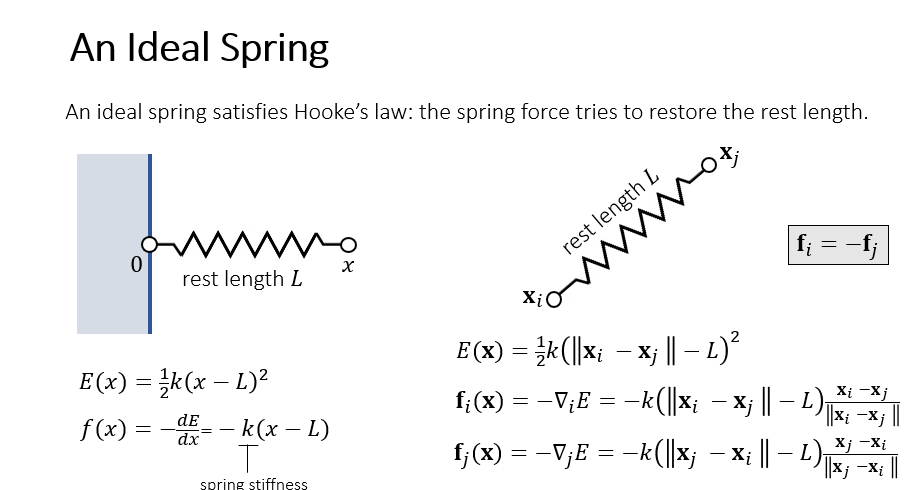
3 Mass-Spring System

\[\frac{\partial\|\mathbf{x}\|}{\partial\mathbf{x}}=\frac{\partial\left(\mathbf{x}^\mathrm{T}\mathbf{x}\right)^{1/2}}{\partial\mathbf{x}}=\frac{1}{2}\left(\mathbf{x}^\mathrm{T}\mathbf{x}\right)^{-1/2}\frac{\partial\left(\mathbf{x}^\mathrm{T}\mathbf{x}\right)}{\partial\mathbf{x}}=\frac{1}{2\|\mathbf{x}\|}2\mathbf{x}^\mathrm{T}=\frac{\mathbf{x}^\mathrm{T}}{\|\mathbf{x}\|} \]

\[\frac{\partial\left(\mathbf{x}^\mathrm{T}\mathbf{x}\right)}{\partial\mathbf{x}} \]

3.1 Matrix calculus

\[\mathbf u=\mathbf u(\mathbf x),\mathbf v=\mathbf v(\mathbf x) \]

\[\frac{\partial(\mathbf{u}\cdot\mathbf{v})}{\partial\mathbf{x}}=\frac{\partial\mathbf{u}^\top\mathbf{v}}{\partial\mathbf{x}} = \mathbf{u}^{\top}{\frac{\partial\mathbf{v}}{\partial\mathbf{x}}}+\mathbf{v}^{\top}{\frac{\partial\mathbf{u}}{\partial\mathbf{x}}} \]

\[\frac{\partial \mathbf{x}}{\partial \mathbf{x}}=\mathbb{I} \]

\[\frac{\partial\mathbf{u}}{\partial\mathbf{x}},\frac{\partial\mathbf{v}}{\partial\mathbf{x}}\text{in numerator layout} \]

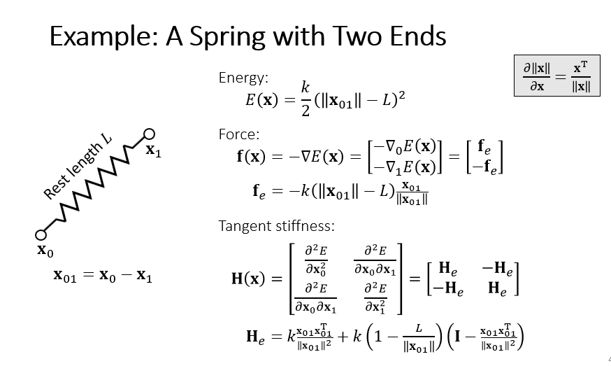
3.2 A Spring with Two Ends

图片来源：Games103

4 Explaination of Init Code with 3D Image

4.1 Initialize

void Start()
{
	Mesh mesh = GetComponent<MeshFilter> ().mesh;

	//Resize the mesh.
	int n=21;
	Vector3[] X  	= new Vector3[n*n];
	Vector2[] UV 	= new Vector2[n*n];
	int[] triangles	= new int[(n-1)*(n-1)*6];
	for(int j=0; j<n; j++)
		for(int i=0; i<n; i++)
		{
			X[j*n+i] =new Vector3(5-10.0f*i/(n-1), 0, 5-10.0f*j/(n-1));
			UV[j*n+i]=new Vector3(i/(n-1.0f), j/(n-1.0f));
		}
	int t=0;
	for(int j=0; j<n-1; j++)
		for(int i=0; i<n-1; i++)
		{
			triangles[t*6+0]=j*n+i;
			triangles[t*6+1]=j*n+i+1;
			triangles[t*6+2]=(j+1)*n+i+1;
			triangles[t*6+3]=j*n+i;
			triangles[t*6+4]=(j+1)*n+i+1;
			triangles[t*6+5]=(j+1)*n+i;
			t++;
		}
	mesh.vertices=X;
	mesh.triangles=triangles;
	mesh.uv = UV;
	mesh.RecalculateNormals ();

	Debug.Log("triangles.Length " + triangles.Length);

	//Construct the original E
	int[] _E = new int[triangles.Length*2];

	Debug.Log("_E.Length " + _E.Length);
	for (int i=0; i<triangles.Length; i+=3) 
	{
		_E[i*2+0]=triangles[i+0];
		_E[i*2+1]=triangles[i+1];
		_E[i*2+2]=triangles[i+1];
		_E[i*2+3]=triangles[i+2];
		_E[i*2+4]=triangles[i+2];
		_E[i*2+5]=triangles[i+0];
	}
	//Reorder the original edge list
	for (int i=0; i<_E.Length; i+=2)
		if(_E[i] > _E[i + 1]) 
			Swap(ref _E[i], ref _E[i+1]);
	//Sort the original edge list using quicksort
	// One edge have two end point, this quicksort method sort all of them at the same time
	// the order is from small to big with the pattern of
	// [start end] [start end] [start end]

	//Debug.Log("_E.Length/2-1 " + (_E.Length / 2 - 1) );
	Quick_Sort(ref _E, 0, _E.Length/2-1);

	// short-circuit evaluation: or(if first condition is true then skip other) and(if first condition is false then skip other)
	int e_number = 0;
	for (int i=0; i<_E.Length; i+=2)
		if (i == 0 || _E [i + 0] != _E [i - 2] || _E [i + 1] != _E [i - 1]) 
			e_number++;

	E = new int[e_number * 2];
	for (int i=0, e=0; i<_E.Length; i+=2)
		if (i == 0 || _E [i + 0] != _E [i - 2] || _E [i + 1] != _E [i - 1]) 
		{
			E[e*2+0]=_E [i + 0];
			E[e*2+1]=_E [i + 1];
			e++;
		}

	// [0-9] 10/2=5 <5=4 4*2+1=9
	// [0-10] 11/2=5 <5=4 4*2+1=9
	// asert(E.length % 2 == 0) this should always be true, becuase we use one dim array to store the Edges. One edge takes two places in this array.
	L = new float[E.Length/2];
	for (int e=0; e<E.Length/2; e++) 
	{
		int v0 = E[e*2+0];
		int v1 = E[e*2+1];
		L[e]=(X[v0]-X[v1]).magnitude;
	}

	V = new Vector3[X.Length];
	for (int i=0; i<V.Length; i++)
		V[i] = new Vector3 (0, 0, 0);
}

4.2 Index

int t=0;
// Because of 21 points have 20 gaps, this index will iterate 400 squares and split them two triangels
// per square.
for(int j=0; j<n-1; j++)
for(int i=0; i<n-1; i++)
{
	triangles[t*6+0]=j*n+i;
	triangles[t*6+1]=j*n+i+1;
	triangles[t*6+2]=(j+1)*n+i+1;
	triangles[t*6+3]=j*n+i;
	triangles[t*6+4]=(j+1)*n+i+1;
	triangles[t*6+5]=(j+1)*n+i;
	t++;
}

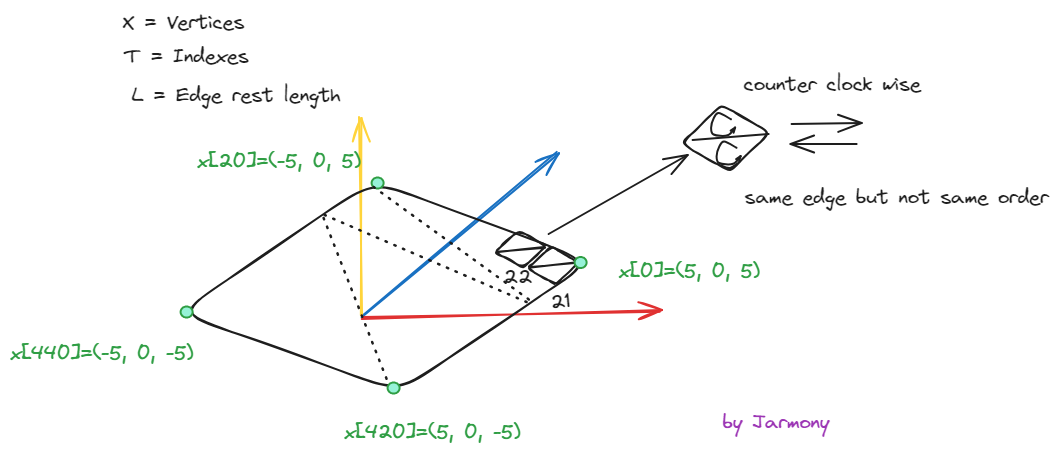
这里的 triangles 其实就是 三角形顶点的Index(下标)。

State: j=0, i=0, t=0.
t[0] = 0
t[1] = 1
t[2] = 22
t[3] = 0
t[4] = 22
t[5] = 21

/*********/

State: j=0, i=1, t=1.
t[6] = 1
t[7] = 2
t[8] = 23
t[9] = 1
t[10] = 23
t[11] = 22

4.3 Edge

//Construct the original E
int[] _E = new int[triangles.Length*2];

Debug.Log("_E.Length " + _E.Length);
for (int i=0; i<triangles.Length; i+=3) 
{
	_E[i*2+0]=triangles[i+0];
	_E[i*2+1]=triangles[i+1];
	
	_E[i*2+2]=triangles[i+1];
	_E[i*2+3]=triangles[i+2];
	
	_E[i*2+4]=triangles[i+2];
	_E[i*2+5]=triangles[i+0];
}
//Reorder the original edge list
for (int i=0; i<_E.Length; i+=2)
	if(_E[i] > _E[i + 1]) 
		Swap(ref _E[i], ref _E[i+1]);

因为这里使用一维数组进行边的存储，那么从一条边到另一条边的步长是2。

State: i=0.
_E[0] = t[0]:0
_E[1] = t[1]:1
_E[2] = t[1]:1
_E[3] = t[2]:22
_E[4] = t[2]:22
_E[5] = t[0]:0

/*********/

State: i=3.
_E[6]= t[3]:0
_E[7] = t[4]:22
_E[8] = t[4]:22
_E[9] = t[5]:21
_E[10] = t[5]:21
_E[11] = t[3]:0

4.4 Sort Edge

//Reorder the original edge list
	for (int i=0; i<_E.Length; i+=2)
		if(_E[i] > _E[i + 1]) 
			Swap(ref _E[i], ref _E[i+1]);

初始的时候，一条边有两种表达方式。我们将其都按从小的顶点到大的顶点进行重新排序，一条边就只有一种表达方式。

Quick_Sort(ref _E, 0, _E.Length/2-1);

void Quick_Sort(ref int[] a, int l, int r)
{
	int j;
	if(l<r)
	{
		j=Quick_Sort_Partition(ref a, l, r);
		Quick_Sort (ref a, l, j-1);
		Quick_Sort (ref a, j+1, r);
	}
}

int  Quick_Sort_Partition(ref int[] a, int l, int r)
{
	int pivot_0, pivot_1, i, j;
	pivot_0 = a [l * 2 + 0];
	pivot_1 = a [l * 2 + 1];
	i = l;
	j = r + 1;
	//Debug.Log("i: " + i + " j:" + j);
	while (true)
	{
		do ++i; while( i<=r && (a[i*2]<pivot_0 || a[i*2]==pivot_0 && a[i*2+1]<=pivot_1));
		do --j; while(  a[j*2]>pivot_0 || a[j*2]==pivot_0 && a[j*2+1]> pivot_1);
		if(i>=j)	break;
		Swap(ref a[i*2], ref a[j*2]);
		Swap(ref a[i*2+1], ref a[j*2+1]);
	}
	Swap (ref a [l * 2 + 0], ref a [j * 2 + 0]);
	Swap (ref a [l * 2 + 1], ref a [j * 2 + 1]);
	return j;
}

void Swap(ref int a, ref int b)
{
	int temp = a;
	a = b;
	b = temp;
}

这里的quick sort是以两个数为一次比较的依据，好像是这两个数打包(其实就是一条边)进行比较，平常就是一次比较只关心一个数。

5 Update

// Update is called once per frame
void Update () 
{
	Mesh mesh = GetComponent<MeshFilter> ().mesh;
	Vector3[] X 		= mesh.vertices;
	Vector3[] last_X 	= new Vector3[X.Length];
	Vector3[] X_hat 	= new Vector3[X.Length];
	Vector3[] G 		= new Vector3[X.Length];

	//Initial Setup.
	for (int i = 0; i < X.Length; i++) 
	{
        if (i == 0 || i == 20) continue;
        V[i] = V[i] * damping;
		X_hat[i] = X[i] + V[i] * t;
		last_X[i] = X[i];
		
		// Guess X[i] init state
		X[i] = X_hat[i];
    }


    float invSquareDt = 1 / (t * t);
	// Hessian Matrix is complicated to construct
	// So we use some fake inverse, due to the mass is same for all vertices, we put this out of the loop.
    float fakeInv = 1 / (invSquareDt * mass + 4.0f * spring_k);
    for (int k=0; k<32; k++)
	{
		Get_Gradient(X, X_hat, t, G);

        //Update X by gradient.
        
        for (int i = 0; i < X.Length; i++)
        {
            if (i == 0 || i == 20) continue;
            X[i] = X[i] - fakeInv * G[i];
        }

    }

	float invTime = 1.0f / t; 
    for (int i = 0; i < X.Length; i++)
    {
        if (i == 0 || i == 20) continue;
        V[i] = invTime * (X[i] - last_X[i]);
    }

    //Finishing.

    mesh.vertices = X;

	Collision_Handling ();
	mesh.RecalculateNormals ();
}

因为要进行优化，位置迭代，来找到最小值。所以需要一个迭代的初始位置，设置为X_init = X[i] + V[i] * t。也可以不设置，不进行变化。

6 Get_Gradient

void Get_Gradient(Vector3[] X, Vector3[] X_hat, float t, Vector3[] G)
{
	//Momentum and Gravity.
	float invSquareDt = 1 / (t * t);
	for (int i = 0; i < X.Length; i++)
	{
		G[i] = invSquareDt * mass * (X[i] - X_hat[i]) - mass * gravity;
    }

	//Spring Force.
	Vector3 spForceDir = Vector3.zero;
	Vector3 spForce = Vector3.zero;

    for (int e = 0; e < E.Length / 2; e++) 
	{
        int vi = E[e * 2 + 0];
        int vj = E[e * 2 + 1];

        spForceDir = X[vi] - X[vj];
		spForce = spring_k * (1.0f - L[e] / spForceDir.magnitude) * spForceDir;
		G[vi] = G[vi] + spForce;
		G[vj] = G[vj] - spForce;
    }
}

6.1 first derivative

\[\mathbf{g}=\frac{1}{\Delta t^2}\mathbf{M}(\mathbf{x}-\tilde{\mathbf{x}})-\mathbf{f}(\mathbf{x}), \]

由于上式的特性，我们需要两次遍历来得到梯度一阶导的数值。

• 逐顶点

\[\mathbf{g}_{i}\leftarrow\frac{1}{\Delta t^{2}}\mathbf{m}_{i}(\mathbf{x}_{i}-\tilde{\mathbf{x}}_{i}). \]

• 逐边计算弹簧弹力

\[\left.\left\{\begin{array}{l}\mathbf{g}_i\leftarrow\mathbf{g}_i+k(1-\frac{L_e}{\|\mathbf{x}_i-\mathbf{x}_j\|})(\mathbf{x}_i-\mathbf{x}_j)\\\mathbf{g}_j\leftarrow\mathbf{g}_j-k(1-\frac{L_e}{\|\mathbf{x}_i-\mathbf{x}_j\|})(\mathbf{x}_i-\mathbf{x}_j)\end{array}\right.\right.. \]

当然无论是逐顶点还是逐边，导数都是位置的函数。

最后给每一个顶点的梯度加上重力，当然根据 g 需要加负号。

6.2 second derivative

In reality, there are two roadblocks:
1)The Hessian matrix is complicated to construct;
2) the linear solver is difficult to implement on Unity.
Instead, we choose a much simpler method by considering the Hessian as a diagonal matrix. This
yields a simple update to every vertex as:

\[\mathbf{x}_{i}\leftarrow\mathbf{x}_{i}-\left(\frac{1}{\Delta t^{2}}m_{i}+4k\right)^{-1}\mathbf{g}_{i}. \]

Games103 Huamin Wang Lab2

7 Collision_Handling

void Collision_Handling()
{
	Mesh mesh = GetComponent<MeshFilter> ().mesh;
	Vector3[] X = mesh.vertices;

	//Handle colllision.
	Vector3 ballPos = GameObject.Find("Sphere").transform.position;
	float radius = 2.7f;

	for (int i = 0; i < X.Length; i++) 
	{
		if (i == 0 || i == 20) continue;
		if (SDF(X[i], ballPos)) 
		{
			V[i] = V[i] + 1.0f / t * (ballPos + radius * (X[i] - ballPos).normalized - X[i]);
			X[i] = ballPos + radius * (X[i] - ballPos).normalized;
		}
	}
}

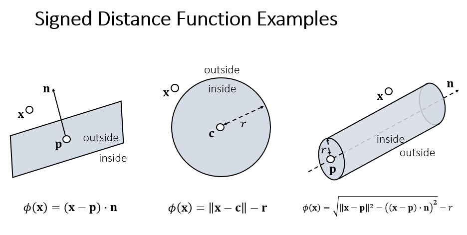
bool SDF(Vector3 v, Vector3 center, float radius = 2.7f) 
{

	float sdf = (v - center).magnitude - radius;
	return sdf > 0.0f ? false : true;
}

Once a colliding vertex is found, apply impulse-based method as follows:

\[\mathbf{v}_i\leftarrow\mathbf{v}_i+\frac{1}{\Delta t}\left(\mathbf{c}+r\frac{\mathbf{x}_i-\mathbf{c}}{\|\mathbf{x}_i-\mathbf{c}\|}-\mathbf{x}_i\right),\quad\mathbf{x}_i\leftarrow\mathbf{c}+r\frac{\mathbf{x}_i-\mathbf{c}}{\|\mathbf{x}_i-\mathbf{c}\|}. \]

图片来源：Games103