Focal Loss 损失函数简述

Focal Loss

摘要

Focal Loss目标是解决样本类别不平衡以及样本分类难度不平衡等问题，如目标检测中大量简单的background，很少量较难的foreground样本。Focal Loss通过修改交叉熵函数，通过增加类别权重\(\alpha\) 和 样本难度权重调因子(modulating factor)\((1-p_t)^\gamma\)，来减缓上述问题，提升模型精确。

一、技术背景

我们知道object detection的算法主要可以分为两大类：two-stage detector和one-stage detector。前者是指类似Faster RCNN，RFCN这样需要region proposal的检测算法，这类算法可以达到很高的准确率，但是速度较慢。虽然可以通过减少proposal的数量或降低输入图像的分辨率等方式达到提速，但是速度并没有质的提升。后者是指类似YOLO，SSD这样不需要region proposal，直接回归的检测算法，这类算法速度很快，但是准确率不如前者。作者提出focal loss的出发点也是希望one-stage detector可以达到two-stage detector的准确率，同时不影响原有的速度。

二、拟解决问题

作者认为one-stage detector的准确率不如two-stage detector的原因是：样本不均衡问题，其中包括两个方面：

• 1. 解决样本的类别不平衡问题
• 2. 解决简单/困难样本不平衡问题

When summed over a lager number of easy examples, these small loss values can overwhelm the rare class.
大量loss小的简单样本相加，可以淹没稀有类.

如在object detection领域，一张图像可能生成成千上万的candidate locations，但是其中只有很少一部分是包含object的（1：1000）。这就带来了类别不均衡。那么类别不均衡会带来什么后果呢？引用原文讲的两个后果：(1) training is inefficient as most locations are easy negatives that contribute no useful learning signal; (2) en masse, the easy negatives can overwhelm training and lead to degenerate models.
负样本数量太大，占总的loss的大部分，而且多是容易分类的，因此使得模型的优化方向并不是我们所希望的那样。

三、解决方案

为了解决（1）解决样本的类别不平衡问题和（2）解决简单/困难样本不平衡问题，作者提出一种新的损失函数：focal loss。这个损失函数是在标准交叉熵损失基础上改进得到：

该focal loss函数曲线为：

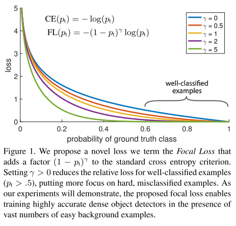
其中，\(-log(p_t)\) 为初始交叉熵损失函数，\(\alpha\) 为类别间（0-1二分类）的权重参数，\((1-p_t)^\gamma\) 为简单/困难样本调节因子（modulating factor），而\(\gamma\) 则聚焦参数（focusing parameter）。

1、形成过程：

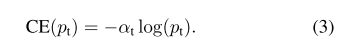
（1）初始二分类的交叉熵（Cross Emtropy, CE）函数：

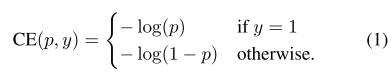
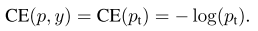
在上面的\(y\in \{\pm1\}\) 为指定的ground-truth类别，\(p \in [0, 1]\) 是模型对带有 \(y=1\) 标签类别的概率估计。为了方便，我们将\(p_t\)定义为：

和重写的\(CE(p, y)\)：

（2）平衡交叉熵（Balanced Cross Entropy）：

一个普遍解决类别不平衡的方法是增加权重参数\(\alpha \in [0 ,1]\)，当$ y=1 \(类的权重为\)\alpha$ ，\(y=-1\) 类的权重为\(1-\alpha\) 。在实验中，\(\alpha\) 被设成逆类别频率（inverse class frequence），\(\alpha_t\)定义与\(p_t\)一样：

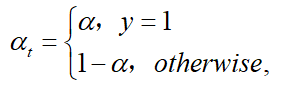
因此，\(\alpha-balanced\) 的CE损失函数为：

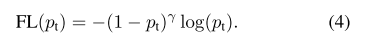
（3）聚焦损失（Focal Loss）：

尽管\(\alpha\)能平衡positive/negative的重要性，但是无法区分简单easy/困难hard样本。为此，对于简单的样本增加一个小的权重(down-weighted)，让损失函数聚焦在困难样本的训练。
因此，在交叉熵损失函数增加调节因子\((1-p_t)^\gamma\) ，和可调节聚参数\(\gamma \geq 0\)。，所以损失函数变成：

当\(p_t\rightarrow0\)时，同时调节因子也 \((1-p_t)^\gamma\rightarrow0\) ，因此简单样本的权重越小。直观地讲，调节因子减少了简单示例的loss贡献，并扩展了样本接收低loss的范围。 例如，在γ= 2的情况下，与CE相比，分类为pt = 0.9的示例的损失将降低100倍，而对于pt≈0.968的示例，其损失将降低1000倍。 这反过来增加了纠正错误分类示例的重要性（对于pt≤0.5和γ= 2，其损失最多缩小4倍）。

（4）最终的损失函数Focal Loss形式：

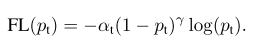
根据论文作者实验，\(\alpha=0.25\) 和 \(\gamma=2\) 效果最好

实现代码：

def focal_loss(y_true, y_pred):
    alpha, gamma = 0.25, 2
    y_pred = K.clip(y_pred, 1e-8, 1 - 1e-8)
    return - alpha * y_true * K.log(y_pred) * (1 - y_pred)**gamma\
           - (1 - alpha) * (1 - y_true) * K.log(1 - y_pred) * y_pred**gamma

四、Reference

1. https://blog.csdn.net/u014380165/article/details/77019084
2. Lin T Y, Goyal P, Girshick R, et al. Focal loss for dense object detection[C]//Proceedings of the IEEE international conference on computer vision. 2017: 2980-2988.