KNN笔记
KNN笔记
先简单加载一下sklearn里的数据集,然后再来讲KNN。
1 import numpy as np
2 import matplotlib as mpl
3 import matplotlib.pyplot as plt
4 from sklearn import datasets
5 iris=datasets.load_iris()
看一下鸢尾花的keys:
iris.keys()
结果是:
dict_keys(['data', 'target', 'target_names', 'DESCR', 'feature_names'])
看一下文档:
print(iris.DESCR) #看看文档
文档结果:


Iris Plants Database
====================

Notes
-----
Data Set Characteristics:
    :Number of Instances: 150 (50 in each of three classes)
    :Number of Attributes: 4 numeric, predictive attributes and the class
    :Attribute Information:
        - sepal length in cm
        - sepal width in cm
        - petal length in cm
        - petal width in cm
        - class:
                - Iris-Setosa
                - Iris-Versicolour
                - Iris-Virginica
    :Summary Statistics:

    ============== ==== ==== ======= ===== ====================
                    Min  Max   Mean    SD   Class Correlation
    ============== ==== ==== ======= ===== ====================
    sepal length:   4.3  7.9   5.84   0.83    0.7826
    sepal width:    2.0  4.4   3.05   0.43   -0.4194
    petal length:   1.0  6.9   3.76   1.76    0.9490  (high!)
    petal width:    0.1  2.5   1.20  0.76     0.9565  (high!)
    ============== ==== ==== ======= ===== ====================

    :Missing Attribute Values: None
    :Class Distribution: 33.3% for each of 3 classes.
    :Creator: R.A. Fisher
    :Donor: Michael Marshall (MARSHALL%PLU@io.arc.nasa.gov)
    :Date: July, 1988

This is a copy of UCI ML iris datasets.
http://archive.ics.uci.edu/ml/datasets/Iris

The famous Iris database, first used by Sir R.A Fisher

This is perhaps the best known database to be found in the
pattern recognition literature.  Fisher's paper is a classic in the field and
is referenced frequently to this day.  (See Duda & Hart, for example.)  The
data set contains 3 classes of 50 instances each, where each class refers to a
type of iris plant.  One class is linearly separable from the other 2; the
latter are NOT linearly separable from each other.

References
----------
   - Fisher,R.A. "The use of multiple measurements in taxonomic problems"
     Annual Eugenics, 7, Part II, 179-188 (1936); also in "Contributions to
     Mathematical Statistics" (John Wiley, NY, 1950).
   - Duda,R.O., & Hart,P.E. (1973) Pattern Classification and Scene Analysis.
     (Q327.D83) John Wiley & Sons.  ISBN 0-471-22361-1.  See page 218.
   - Dasarathy, B.V. (1980) "Nosing Around the Neighborhood: A New System
     Structure and Classification Rule for Recognition in Partially Exposed
     Environments".  IEEE Transactions on Pattern Analysis and Machine
     Intelligence, Vol. PAMI-2, No. 1, 67-71.
   - Gates, G.W. (1972) "The Reduced Nearest Neighbor Rule".  IEEE Transactions
     on Information Theory, May 1972, 431-433.
   - See also: 1988 MLC Proceedings, 54-64.  Cheeseman et al"s AUTOCLASS II
     conceptual clustering system finds 3 classes in the data.
   - Many, many more ...
看一下数据data:
iris.data #看看数据
数据为:
  1 array([[ 5.1,  3.5,  1.4,  0.2],
  2        [ 4.9,  3. ,  1.4,  0.2],
  3        [ 4.7,  3.2,  1.3,  0.2],
  4        [ 4.6,  3.1,  1.5,  0.2],
  5        [ 5. ,  3.6,  1.4,  0.2],
  6        [ 5.4,  3.9,  1.7,  0.4],
  7        [ 4.6,  3.4,  1.4,  0.3],
  8        [ 5. ,  3.4,  1.5,  0.2],
  9        [ 4.4,  2.9,  1.4,  0.2],
 10        [ 4.9,  3.1,  1.5,  0.1],
 11        [ 5.4,  3.7,  1.5,  0.2],
 12        [ 4.8,  3.4,  1.6,  0.2],
 13        [ 4.8,  3. ,  1.4,  0.1],
 14        [ 4.3,  3. ,  1.1,  0.1],
 15        [ 5.8,  4. ,  1.2,  0.2],
 16        [ 5.7,  4.4,  1.5,  0.4],
 17        [ 5.4,  3.9,  1.3,  0.4],
 18        [ 5.1,  3.5,  1.4,  0.3],
 19        [ 5.7,  3.8,  1.7,  0.3],
 20        [ 5.1,  3.8,  1.5,  0.3],
 21        [ 5.4,  3.4,  1.7,  0.2],
 22        [ 5.1,  3.7,  1.5,  0.4],
 23        [ 4.6,  3.6,  1. ,  0.2],
 24        [ 5.1,  3.3,  1.7,  0.5],
 25        [ 4.8,  3.4,  1.9,  0.2],
 26        [ 5. ,  3. ,  1.6,  0.2],
 27        [ 5. ,  3.4,  1.6,  0.4],
 28        [ 5.2,  3.5,  1.5,  0.2],
 29        [ 5.2,  3.4,  1.4,  0.2],
 30        [ 4.7,  3.2,  1.6,  0.2],
 31        [ 4.8,  3.1,  1.6,  0.2],
 32        [ 5.4,  3.4,  1.5,  0.4],
 33        [ 5.2,  4.1,  1.5,  0.1],
 34        [ 5.5,  4.2,  1.4,  0.2],
 35        [ 4.9,  3.1,  1.5,  0.1],
 36        [ 5. ,  3.2,  1.2,  0.2],
 37        [ 5.5,  3.5,  1.3,  0.2],
 38        [ 4.9,  3.1,  1.5,  0.1],
 39        [ 4.4,  3. ,  1.3,  0.2],
 40        [ 5.1,  3.4,  1.5,  0.2],
 41        [ 5. ,  3.5,  1.3,  0.3],
 42        [ 4.5,  2.3,  1.3,  0.3],
 43        [ 4.4,  3.2,  1.3,  0.2],
 44        [ 5. ,  3.5,  1.6,  0.6],
 45        [ 5.1,  3.8,  1.9,  0.4],
 46        [ 4.8,  3. ,  1.4,  0.3],
 47        [ 5.1,  3.8,  1.6,  0.2],
 48        [ 4.6,  3.2,  1.4,  0.2],
 49        [ 5.3,  3.7,  1.5,  0.2],
 50        [ 5. ,  3.3,  1.4,  0.2],
 51        [ 7. ,  3.2,  4.7,  1.4],
 52        [ 6.4,  3.2,  4.5,  1.5],
 53        [ 6.9,  3.1,  4.9,  1.5],
 54        [ 5.5,  2.3,  4. ,  1.3],
 55        [ 6.5,  2.8,  4.6,  1.5],
 56        [ 5.7,  2.8,  4.5,  1.3],
 57        [ 6.3,  3.3,  4.7,  1.6],
 58        [ 4.9,  2.4,  3.3,  1. ],
 59        [ 6.6,  2.9,  4.6,  1.3],
 60        [ 5.2,  2.7,  3.9,  1.4],
 61        [ 5. ,  2. ,  3.5,  1. ],
 62        [ 5.9,  3. ,  4.2,  1.5],
 63        [ 6. ,  2.2,  4. ,  1. ],
 64        [ 6.1,  2.9,  4.7,  1.4],
 65        [ 5.6,  2.9,  3.6,  1.3],
 66        [ 6.7,  3.1,  4.4,  1.4],
 67        [ 5.6,  3. ,  4.5,  1.5],
 68        [ 5.8,  2.7,  4.1,  1. ],
 69        [ 6.2,  2.2,  4.5,  1.5],
 70        [ 5.6,  2.5,  3.9,  1.1],
 71        [ 5.9,  3.2,  4.8,  1.8],
 72        [ 6.1,  2.8,  4. ,  1.3],
 73        [ 6.3,  2.5,  4.9,  1.5],
 74        [ 6.1,  2.8,  4.7,  1.2],
 75        [ 6.4,  2.9,  4.3,  1.3],
 76        [ 6.6,  3. ,  4.4,  1.4],
 77        [ 6.8,  2.8,  4.8,  1.4],
 78        [ 6.7,  3. ,  5. ,  1.7],
 79        [ 6. ,  2.9,  4.5,  1.5],
 80        [ 5.7,  2.6,  3.5,  1. ],
 81        [ 5.5,  2.4,  3.8,  1.1],
 82        [ 5.5,  2.4,  3.7,  1. ],
 83        [ 5.8,  2.7,  3.9,  1.2],
 84        [ 6. ,  2.7,  5.1,  1.6],
 85        [ 5.4,  3. ,  4.5,  1.5],
 86        [ 6. ,  3.4,  4.5,  1.6],
 87        [ 6.7,  3.1,  4.7,  1.5],
 88        [ 6.3,  2.3,  4.4,  1.3],
 89        [ 5.6,  3. ,  4.1,  1.3],
 90        [ 5.5,  2.5,  4. ,  1.3],
 91        [ 5.5,  2.6,  4.4,  1.2],
 92        [ 6.1,  3. ,  4.6,  1.4],
 93        [ 5.8,  2.6,  4. ,  1.2],
 94        [ 5. ,  2.3,  3.3,  1. ],
 95        [ 5.6,  2.7,  4.2,  1.3],
 96        [ 5.7,  3. ,  4.2,  1.2],
 97        [ 5.7,  2.9,  4.2,  1.3],
 98        [ 6.2,  2.9,  4.3,  1.3],
 99        [ 5.1,  2.5,  3. ,  1.1],
100        [ 5.7,  2.8,  4.1,  1.3],
101        [ 6.3,  3.3,  6. ,  2.5],
102        [ 5.8,  2.7,  5.1,  1.9],
103        [ 7.1,  3. ,  5.9,  2.1],
104        [ 6.3,  2.9,  5.6,  1.8],
105        [ 6.5,  3. ,  5.8,  2.2],
106        [ 7.6,  3. ,  6.6,  2.1],
107        [ 4.9,  2.5,  4.5,  1.7],
108        [ 7.3,  2.9,  6.3,  1.8],
109        [ 6.7,  2.5,  5.8,  1.8],
110        [ 7.2,  3.6,  6.1,  2.5],
111        [ 6.5,  3.2,  5.1,  2. ],
112        [ 6.4,  2.7,  5.3,  1.9],
113        [ 6.8,  3. ,  5.5,  2.1],
114        [ 5.7,  2.5,  5. ,  2. ],
115        [ 5.8,  2.8,  5.1,  2.4],
116        [ 6.4,  3.2,  5.3,  2.3],
117        [ 6.5,  3. ,  5.5,  1.8],
118        [ 7.7,  3.8,  6.7,  2.2],
119        [ 7.7,  2.6,  6.9,  2.3],
120        [ 6. ,  2.2,  5. ,  1.5],
121        [ 6.9,  3.2,  5.7,  2.3],
122        [ 5.6,  2.8,  4.9,  2. ],
123        [ 7.7,  2.8,  6.7,  2. ],
124        [ 6.3,  2.7,  4.9,  1.8],
125        [ 6.7,  3.3,  5.7,  2.1],
126        [ 7.2,  3.2,  6. ,  1.8],
127        [ 6.2,  2.8,  4.8,  1.8],
128        [ 6.1,  3. ,  4.9,  1.8],
129        [ 6.4,  2.8,  5.6,  2.1],
130        [ 7.2,  3. ,  5.8,  1.6],
131        [ 7.4,  2.8,  6.1,  1.9],
132        [ 7.9,  3.8,  6.4,  2. ],
133        [ 6.4,  2.8,  5.6,  2.2],
134        [ 6.3,  2.8,  5.1,  1.5],
135        [ 6.1,  2.6,  5.6,  1.4],
136        [ 7.7,  3. ,  6.1,  2.3],
137        [ 6.3,  3.4,  5.6,  2.4],
138        [ 6.4,  3.1,  5.5,  1.8],
139        [ 6. ,  3. ,  4.8,  1.8],
140        [ 6.9,  3.1,  5.4,  2.1],
141        [ 6.7,  3.1,  5.6,  2.4],
142        [ 6.9,  3.1,  5.1,  2.3],
143        [ 5.8,  2.7,  5.1,  1.9],
144        [ 6.8,  3.2,  5.9,  2.3],
145        [ 6.7,  3.3,  5.7,  2.5],
146        [ 6.7,  3. ,  5.2,  2.3],
147        [ 6.3,  2.5,  5. ,  1.9],
148        [ 6.5,  3. ,  5.2,  2. ],
149        [ 6.2,  3.4,  5.4,  2.3],
150        [ 5.9,  3. ,  5.1,  1.8]])
可见data为150行,每行4列的数据。
看一下target:
iris.target #看看对应的目标值
target结果为:
array([0, 0, 0, 0, 0, 0, 0, 0, 0, 0, 0, 0, 0, 0, 0, 0, 0, 0, 0, 0, 0, 0, 0,
       0, 0, 0, 0, 0, 0, 0, 0, 0, 0, 0, 0, 0, 0, 0, 0, 0, 0, 0, 0, 0, 0, 0,
       0, 0, 0, 0, 1, 1, 1, 1, 1, 1, 1, 1, 1, 1, 1, 1, 1, 1, 1, 1, 1, 1, 1,
       1, 1, 1, 1, 1, 1, 1, 1, 1, 1, 1, 1, 1, 1, 1, 1, 1, 1, 1, 1, 1, 1, 1,
       1, 1, 1, 1, 1, 1, 1, 1, 2, 2, 2, 2, 2, 2, 2, 2, 2, 2, 2, 2, 2, 2, 2,
       2, 2, 2, 2, 2, 2, 2, 2, 2, 2, 2, 2, 2, 2, 2, 2, 2, 2, 2, 2, 2, 2, 2,
       2, 2, 2, 2, 2, 2, 2, 2, 2, 2, 2, 2])
看一下target_names:
iris.target_names #看看目标值对应的目标名称
arget_names结果为:
array(['setosa', 'versicolor', 'virginica'],
      dtype='<U10')
也就是target的0,1,2分别对应的鸢尾花的名称就是这三个。
看一下4列数据(也就是data)分别是指什么
iris.feature_names #看看四个数据对应的是什么
可以看到结果为:
['sepal length (cm)',
 'sepal width (cm)',
 'petal length (cm)',
 'petal width (cm)']
也就是4列数据分别代表花萼的长,花萼的宽,花瓣的长,花瓣的宽。
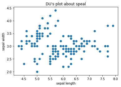
看一下花萼的数据,也就是前两列的数据:
1 #看一下花萼的散点图
2 X=iris.data[:,:2]
3 plt.scatter(X[:,0],X[:,1])
4 plt.xlabel("sepal length")
5 plt.ylabel("sepal width")
6 plt.title("DU's plot about speal")
7 plt.show()
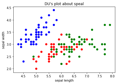
把三种花的散点图区分一下:
1 #把三种花的花萼的散点图画出来
2 y=iris.target
3 plt.scatter(X[y==0,0],X[y==0,1],color='b')
4 plt.scatter(X[y==1,0],X[y==1,1],color='r')
5 plt.scatter(X[y==2,0],X[y==2,1],color='g')
6 plt.xlabel("sepal length")
7 plt.ylabel("sepal width")
8 plt.title("DU's plot about speal")
9 plt.show()
再看一下花瓣的散点图:
1 Petal=iris.data[:,2:]
2 y=iris.target
3 plt.scatter(Petal[y==0,0],Petal[y==0,1],color='b')
4 plt.scatter(Petal[y==1,0],Petal[y==1,1],color='r')
5 plt.scatter(Petal[y==2,0],Petal[y==2,1],color='g')
6 plt.xlabel("Petal length")
7 plt.ylabel("Petal width")
8 plt.title("DU's plot about Petal")
9 plt.show()
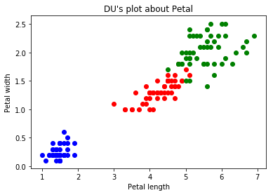
看到花瓣的散点图,那么就说一下KNN,那现在假设,花瓣散点图里来了一个长度为2cm,宽度主0.5cm的一个点,那么这个点代表的是哪个鸢尾呢?一般的人就能推出这个点应该是跟蓝色点是一类的,因为新进来的点是离蓝色的区域最近的,而离其他的红色或者绿色区域都很远。那么,这就是KNN的一个思想了。
比如现假设有如下场景,模拟有如下数据:
 1 raw_X=[[1,2],
 2        [2.8,2.5],
 3        [4,3.2],
 4        [2,1.5],
 5        [6,7.8],
 6        [8,5],
 7        [9,7],
 8        [7,8.5],
 9        [10,9.7],
10       ]
11 raw_y=[0,0,0,0,1,1,1,1,1]
12 X_train=np.array(raw_X)
13 y_train=np.array(raw_y)
现在有一个数据x(设置为绿色的点)进来了,要判断这个数据是属于哪一类的:
1 x=np.array([7.5,6.5])
2 plt.scatter(X_train[y_train==0,0],X_train[y_train==0,1])
3 plt.scatter(X_train[y_train==1,0],X_train[y_train==1,1],color='r')
4 plt.scatter(x[0],x[1],color='g')
5 plt.show()
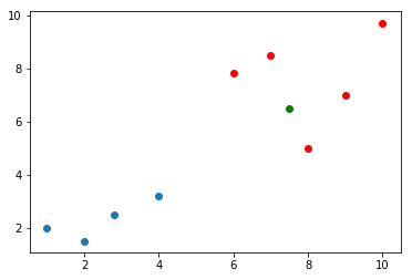
那么,按照KNN的思路就需求,求出这个里面,所有点离这个绿色点的距离了,看这个绿色的点离哪些是最近的。
那么,根据欧拉距离,一般程序员就可以写出这样的代码了:
1 from math import sqrt
2 distances=[]
3 for x_train in X_train:
4     d=sqrt(np.sum(x_train-x)**2)
5     distances.append(d)
当然,根据欧拉距离,不一般的程序员是会这么写:
distances=[sqrt(np.sum(x_train-x)**2) for x_train in X_train]
而结果distances都会是:
[11.0, 8.7, 6.8, 10.5, 0.20000000000000018, 1.0, 2.0, 1.5, 5.699999999999999]
接着,算出距离最近元素的索引,进而拿到距离最近的值:
1 nearest=np.argsort(distances)
2 topK_y=[y_train[i] for neighbor in nearest[:5]]
3 from collections import Counter
4 votes=Counter(topK_y)
5 predict_y=votes.most_common(1)[0][0]
6 predict_y
结果明显是1。

 浙公网安备 33010602011771号