

威斯康星乳腺癌良性预测
一、获取数据
wget https://archive.ics.uci.edu/ml/machine-learning-databases/breast-cancer-wisconsin/breast-cancer-wisconsin.data
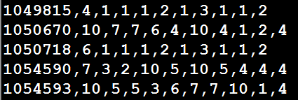
原始数据以逗号分隔:
各个列的属性(包括乳房肿块细针抽吸活检图像的数字化的多项测量值,这些值代表出现在数字化图像中的细胞核的特征):
1.Sample Code Number id number
2.Clump Thickness 1 - 10 肿块厚度
3.Uniformity Of Cell Size 1 - 10 细胞大小均一性
4.Uniformity Of Cell Shape 1 - 10 细胞形状的均一性
5.Marginal Adhesion 1 - 10 边缘附着性
6.Single Epithelial Cell Size 1 - 10 单上皮细胞大小
7.Bare Nuclei 1 - 10 裸核
8.Bland Chromatin 1 - 10 布兰染色质
9.Normal Nucleoli 1 - 10 正常核仁
10.Mitoses 1 - 10 有丝分裂
11.Class 2是良性,4是恶性
这些细胞特征得分为1(最接近良性)至10(最接近病变)之间的整数。
任一变量都不能单独作为判别良性或恶性的标准,建模的目的是找到九个细胞特征的某种组合,从而实现对恶性肿瘤的准确预测
早期的检测过程包括检查乳腺组织的异常肿块。如果发现一个肿块,那么就需要进行细针抽吸活检,即利用一根空心针从肿块中提取细胞的一个小样品,然后临床医生在显微镜下检查细胞,从而确定肿块可能是恶性的还是良
如果机器学习能够自动识别癌细胞,那么它将为医疗系统提供相当大的益处,可以让医生在诊断上花更少的时间,而在治疗疾病上花更多的时间
自动化筛查系统还可能通过去除该过程中的内在主观人为因素来提供更高的检测准确性
二、代码实例
准备工作:桌面新建Breast->cd Breast->shift + 右键->在此处新建命令窗口->jupyter notebook->新建MalignentOrBenign脚本:

1)读取数据并去掉数据中的?
import pandas as pd
import numpy as np
#数据没有标题,因此加上参数header
#df = pd.read_csv('https://archive.ics.uci.edu/ml/machine-learning-databases/breast-cancer-wisconsin/breast-cancer-wisconsin.data', header=None)
df = pd.read_csv('breast-cancer-wisconsin.data', header=None)
column_names = ['Sample code number','Clump Thickness','Uniformity of Cell Size',
'Uniformity of Cell Shape','Marginal Adhesion','Single Epithelial Cell Size',
'Bare Nuclei','Bland Chromatin','Normal Nucleoli','Mitoses','Class']
df.columns = column_names
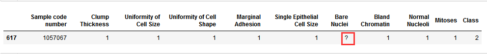
df[df['Sample code number'] == 1057067]
从下面的结果可以看出数据中是存在空值的,只是这个空值是?
我们将?用np.nan填充后,drop掉:
df = df.replace('?', np.nan)
df[df['Sample code number'] == 1057067]

df = df.dropna(how='any')
df[df['Sample code number'] == 1057067]

从上面的结果可以看出?显示被NaN填充,然后该样本被drop掉了
2)数据归一化并拆分数据集
import warnings
warnings.filterwarnings('ignore')

from sklearn.model_selection import train_test_split
from sklearn.preprocessing import StandardScaler
#一般1代表恶性,0代表良性(本数据集4恶性,所以将4变成1,将2变成0)
#df['Class'][data['Class'] == 4] = 1
#df['Class'][data['Class'] == 2] = 0
df.loc[ df['Class'] == 4, 'Class' ] = 1
df.loc[ df['Class'] == 2, 'Class' ] = 0

#Sample code number特征对分类没有作用,将数据集75%作为训练集,25%作为测试集
X_train, X_test, y_train, y_test = train_test_split(df[ column_names[1:10] ], df[ column_names[10] ], test_size = 0.25, random_state = 33)

ss = StandardScaler()
X_train = ss.fit_transform(X_train)
X_test = ss.transform(X_test)
print(X_train[0:5,:])
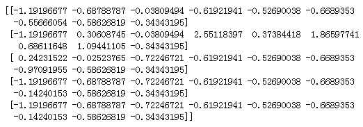
从上面的X_train的前5条数据可以看出数据已经被归一化
3)使用逻辑回归进行分类,并查看其分类正确率
from sklearn.linear_model import LogisticRegression
from sklearn.metrics import accuracy_score
lr = LogisticRegression()
lr.fit(X_train, y_train)
lr_y_predict = lr.predict(X_test)
print( 'The LR Predict Result', accuracy_score(lr_y_predict, y_test) )

#LR也自带了score
print( "The LR Predict Result Show By lr.score", lr.score(X_test, y_test) )
正确率结果如下:

4)使用SGDC进行分类,并查看其分类准确率
from sklearn.linear_model import SGDClassifier
from sklearn.metrics import accuracy_score
sgdc = SGDClassifier()
sgdc.fit(X_train, y_train)
sgdc_y_predict = sgdc.predict(X_test)
print( "The SGDC Predict Result", accuracy_score(sgdc_y_predict, y_test) )
#SGDC也自带了score
print( "The SGDC Predict Result Show By SGDC.score", sgdc.score(X_test, y_test) )
正确率结果如下:

5)利用classification_report查看报告
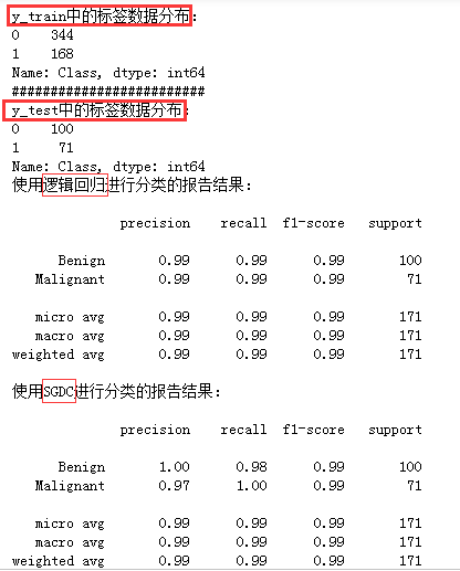
print('y_train中的标签数据分布:')
print(y_train.value_counts())
print( '#' * 25 )
print('y_test中的标签数据分布:')
print(y_test.value_counts())

#分类报告:
from sklearn.metrics import classification_report

#使用classification_report模块获得LR三个指标的结果(召回率,精确率,调和平均数)
print('使用逻辑回归进行分类的报告结果:\n')
print( classification_report( y_test,lr_y_predict,target_names=['Benign','Malignant'] ) )

##使用classification_report模块获得SGDC三个指标的结果
print('使用SGDC进行分类的报告结果:\n')
print( classification_report( y_test,sgdc_y_predict,target_names=['Benign','Malignant'] ) )
代码运行结果如下:
综上:LR和SGDC相比,两者分类效果相同(这里要特别注意:使用SGDC进行分类的结果是不稳定的,每次的结果不一定相同,读者可以多次执行,查看每次的分类结果)
好奇的读者可能会有这样的想法-SGD不是一种随机梯度下降优化算法吗?怎么和分类器搞上关系了呢?
解释如下:原来,随机梯度下降分类器并不是一个独立的算法,而是一系列利用随机梯度下降求解参数的算法的集合
6)使用Xgboost进行分类,并查看分类效果
import xgboost as xgb
from xgboost import XGBClassifier
import matplotlib.pyplot as plt
from sklearn.metrics import accuracy_score
import pandas as pd
from sklearn.model_selection import GridSearchCV
def modelfit(alg, dtrain_x, dtrain_y, useTrainCV=True, cv_flods=5, early_stopping_rounds=50):
"""
:param alg: 初始模型
:param dtrain_x:训练数据X
:param dtrain_y:训练数据y(label)
:param useTrainCV: 是否使用cv函数来确定最佳n_estimators
:param cv_flods:交叉验证的cv数
:param early_stopping_rounds:在该数迭代次数之前,eval_metric都没有提升的话则停止
"""
if useTrainCV:
xgb_param = alg.get_xgb_params()
xgtrain = xgb.DMatrix(dtrain_x, dtrain_y)
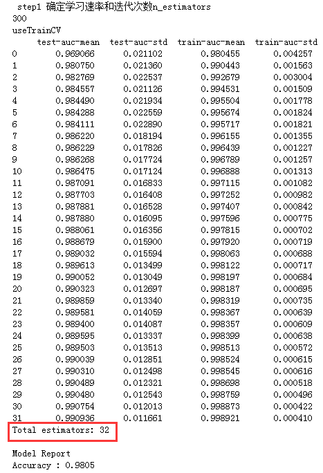
print(alg.get_params()['n_estimators'])
cv_result = xgb.cv( xgb_param, xgtrain, num_boost_round=alg.get_params()['n_estimators'],
nfold=cv_flods, metrics = 'auc', early_stopping_rounds=early_stopping_rounds)
print('useTrainCV\n',cv_result)
print('Total estimators:',cv_result.shape[0])
alg.set_params(n_estimators=cv_result.shape[0])
# train data
alg.fit(X_train, y_train, eval_metric='auc')
#predict train data
train_y_pre = alg.predict(X_train)
print ("\nModel Report")
print ("Accuracy : %.4g" % accuracy_score(y_train, train_y_pre))
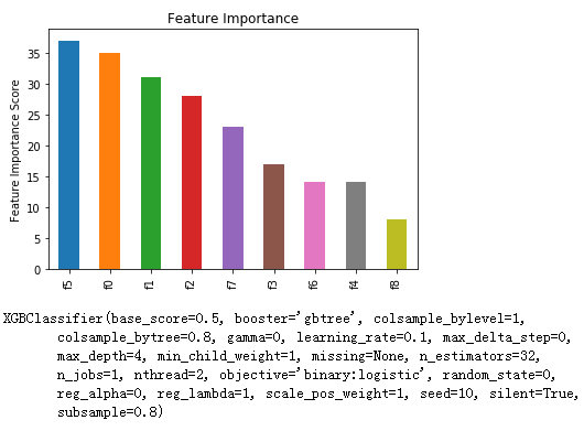
feat_imp = pd.Series( alg.get_booster().get_fscore()).sort_values( ascending=False )
feat_imp.plot( kind = 'bar', title='Feature Importance' )
plt.ylabel('Feature Importance Score')
plt.show()
print(alg)
#XGBoost调参
def xgboost_change_param(train_X, train_y):
print('######Xgboost调参######')
print('\n step1 确定学习速率和迭代次数n_estimators')
xgb1 = XGBClassifier(learning_rate=0.1, booster='gbtree', n_estimators=300,
max_depth=4, min_child_weight=1,
gamma=0, subsample=0.8, colsample_bytree=0.8,
objective='binary:logistic',
nthread=2, scale_pos_weight=1, seed=10)
#useTrainCV=True时,最佳n_estimators=32, learning_rate=0.1
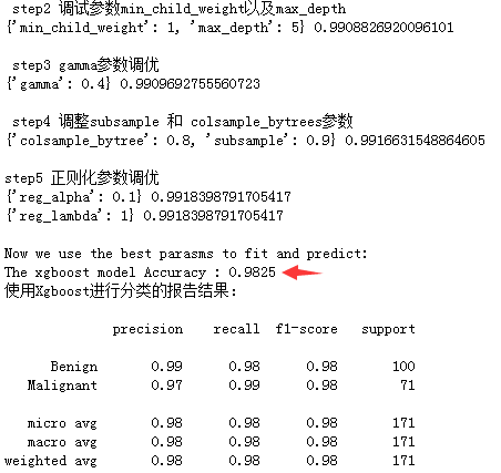
modelfit(xgb1, train_X, train_y, early_stopping_rounds=45)
print('\n step2 调试参数min_child_weight以及max_depth')
param_test1 = { 'max_depth' : range(3, 8, 1), 'min_child_weight' : range(1, 6, 2) }
#GridSearchCV()中的estimator参数所使用的分类器
#并且传入除需要确定最佳的参数之外的其他参数
#每一个分类器都需要一个scoring参数,或者score方法
gsearch1 = GridSearchCV( estimator=XGBClassifier( learning_rate=0.1,n_estimators=32,
gamma=0,
subsample=0.8,colsample_bytree=0.8,
objective='binary:logistic',nthreads=2,
scale_pos_weight=1,seed=10 ),
param_grid=param_test1,scoring='roc_auc',n_jobs=1,cv=5)
gsearch1.fit(train_X,train_y)
#最佳max_depth = 5 min_child_weight=1
print(gsearch1.best_params_, gsearch1.best_score_)
print('\n step3 gamma参数调优')
param_test2 = { 'gamma': [i/10.0 for i in range(0,5)] }
gsearch2 = GridSearchCV( estimator=XGBClassifier(learning_rate=0.1,n_estimators=32,
max_depth=5,min_child_weight=1,
subsample=0.8,colsample_bytree=0.8,
objective='binary:logistic',nthread=2,
scale_pos_weight=1,seed=10),
param_grid=param_test2,scoring='roc_auc',cv=5 )
gsearch2.fit(train_X, train_y)
#最佳 gamma = 0.4
print(gsearch2.best_params_, gsearch2.best_score_)
print('\n step4 调整subsample 和 colsample_bytrees参数')
param_test3 = { 'subsample': [i/10.0 for i in range(6,10)],
'colsample_bytree': [i/10.0 for i in range(6,10)] }
gsearch3 = GridSearchCV( estimator=XGBClassifier(learning_rate=0.1,n_estimators=32,
max_depth=5,min_child_weight=1,gamma=0.4,
objective='binary:logistic',nthread=2,
scale_pos_weight=1,seed=10),
param_grid=param_test3,scoring='roc_auc',cv=5 )
gsearch3.fit(train_X, train_y)
#最佳'subsample': 0.9, 'colsample_bytree': 0.8
print(gsearch3.best_params_, gsearch3.best_score_)
print('\nstep5 正则化参数调优')
param_test4= { 'reg_alpha':[1e-5, 1e-2, 0.1, 1, 100] }
gsearch4= GridSearchCV(estimator=XGBClassifier(learning_rate=0.1,n_estimators=32,
max_depth=5,min_child_weight=1,gamma=0.4,
subsample=0.9,colsample_bytree=0.8,
objective='binary:logistic',nthread=2,
scale_pos_weight=1,seed=10),
param_grid=param_test4,scoring='roc_auc',cv=5 )
gsearch4.fit(train_X, train_y)
#reg_alpha:0.1
print(gsearch4.best_params_, gsearch4.best_score_)
param_test5 ={ 'reg_lambda':[1e-5, 1e-2, 0.1, 1, 100] }
gsearch5= GridSearchCV(estimator=XGBClassifier(learning_rate=0.1,n_estimators=32,
max_depth=5,min_child_weight=1,gamma=0.4,
subsample=0.9,colsample_bytree=0.8,
objective='binary:logistic',nthread=2,reg_alpha=0.1,
scale_pos_weight=1,seed=10),
param_grid=param_test5,scoring='roc_auc',cv=5)
gsearch5.fit(train_X, train_y)
#reg_lambda:1
print(gsearch5.best_params_, gsearch5.best_score_)
# XGBoost调参
xgboost_change_param(X_train, y_train)
#parameters at last
print('\nNow we use the best parasms to fit and predict:')
xgb1 = XGBClassifier(learning_rate=0.1,n_estimators=32,max_depth=5,min_child_weight=1,
gamma=0.4,subsample=0.9,colsample_bytree=0.8,
objective='binary:logistic',reg_alpha=0.1,reg_lambda=1,
nthread=2, scale_pos_weight=1,seed=10)
xgb1.fit(X_train,y_train)
y_test_pre = xgb1.predict(X_test)
y_test_true = y_test
print ("The xgboost model Accuracy : %.4g" % accuracy_score(y_pred=y_test_pre, y_true=y_test_true))
print('使用Xgboost进行分类的报告结果:\n')
print( classification_report( y_test_true,y_test_pre,target_names=['Benign','Malignant'] ) )
下面来看看Xgboost效果如何:
7)使用SVM进行分类,并查看分类效果
from sklearn.svm import SVC
from sklearn.metrics import accuracy_score
models = ( SVC(kernel='rbf', gamma=0.1, C=1.0),
SVC(kernel='rbf', gamma=1, C=1.0),
SVC(kernel='rbf', gamma=10, C=1.0) )
models = ( clf.fit(X_train, y_train) for clf in models )
for clf in models:
clf.fit(X_train, y_train)
y_test_pre = clf.predict(X_test)
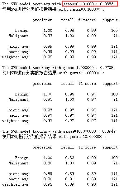
print ("The SVM model Accuracy with gamma=%f : %.4g" % (clf.gamma,accuracy_score(y_pred=y_test_pre, y_true=y_test)) )
print('使用SVM进行分类的报告结果 with gamma=%f :\n' % clf.gamma)
print( classification_report( y_test,y_test_pre,target_names=['Benign','Malignant'] ) )
我们设置了gamma参数,其分类效果如下,最佳结果还是gamm=0.1
SVM模型有两个非常重要的参数C与gamma。其中 C是惩罚系数,即对误差的宽容度。C越高,说明越不能容忍出现误差,容易过拟合。C越小,容易欠拟合。C过大或过小,泛化能力变差
gamma决定了数据映射到新的特征空间后的分布
通过上面的结果发现Xgboost在本例上并没有体现出优势,并且在还有点过拟合,在训练集上表现比在测试集上结果好

 浙公网安备 33010602011771号