SciTech-BigDataAIML-BackPropagation: 一文搞懂反向传播

SciTech-BigDataAIML-BackPropagation:

一文搞懂BackPropagation(反向传播)

参考文献

Back Propagation is also known as "Backward Propagation of Errors",
which is a method used to train neural network .
Its goal is to reduce the difference between the model’s predicted output and the actual output by adjusting the weights and biases in the network.

It works iteratively to adjust weights and bias to minimize the cost function.
In each epoch the model adapts these parameters by reducing loss by following the error gradient.
It often uses optimization algorithms like gradient descent or stochastic gradient descent. The algorithm computes the gradient using the chain rule from calculus allowing it to effectively navigate complex layers in the neural network to minimize the cost function.

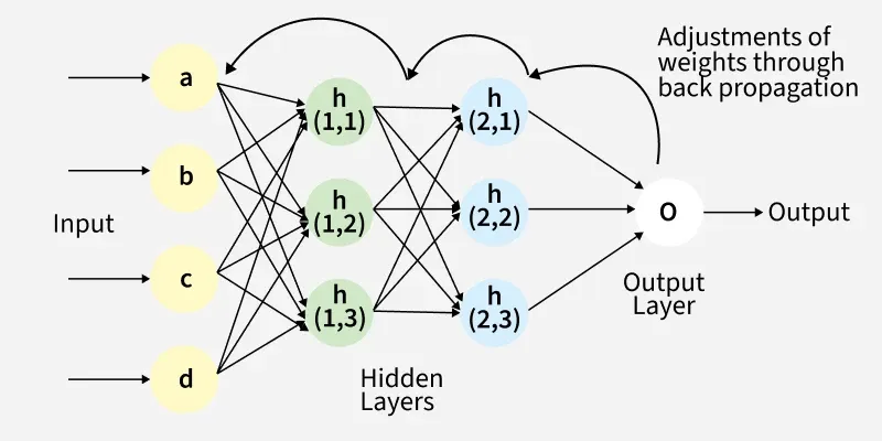
Fig(a): A simple illustration of how the back propagation works by adjustments of weights

Back Propagation plays a critical role in how neural networks improve over time.
Here's why:

Efficient Weight Update: It computes the gradient of the loss function with respect to each weight using the chain rule making it possible to update weights efficiently.
Scalability: The Back Propagation algorithm scales well to networks with multiple layers and complex architectures making deep learning feasible.
Automated Learning: With Back Propagation the learning process becomes automated and the model can adjust itself to optimize its performance.

Working of Back Propagation Algorithm

The Back Propagation algorithm involves two main steps:
the Forward Pass and the Backward Pass.

1. Forward Pass Work

In forward pass the input data is fed into the input layer.
These inputs combined with their respective weights are passed to hidden layers.
For example, in a network with two hidden layers (h1 and h2):

the output from h1 serves as the input to h2.
Before applying an activation function, a bias is added to the weighted inputs.
Each hidden layer computes the weighted sum (a) of the inputs, then applies an activation function like ReLU (Rectified Linear Unit) to obtain the output (o).
The output is passed to the next layer where an activation function such as softmax converts the weighted outputs into probabilities for classification.

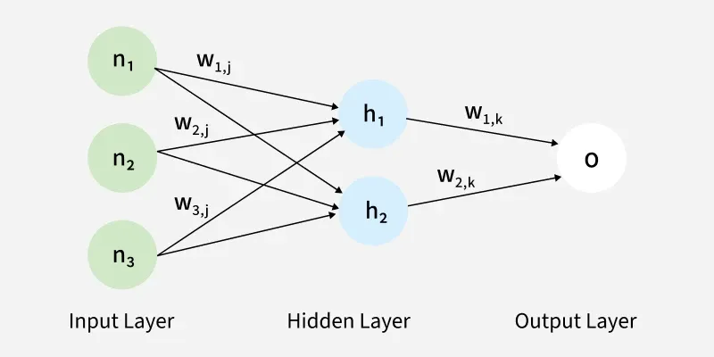
The forward pass using weights and biases

一、前言

这是一场以 Error(误差) 为主导的 Back Propagation(反向传播) 运动，
旨在得到最优的全局参数矩阵，进而将 多层神经网络 用到 Classification(分类)或者 Regression(回归)任务去。

模型:

都有 Parameter Matrix(参数矩阵)、Inputs(输入) 和 Outputs(输出).
可有 [0, N) 层隐藏层; 每一层"隐藏层"都有其直连的Parameter Matrix(参数矩阵)
大多数模型有 Training 和 Predication 两个过程.
Training 过程用 GroundTruth 训练并保存出全局最优的 Parameter Matrix(参数矩阵);
Predication 过程则直接用保存好的全局最优 Parameter Matrix 运行训练好的模型.
Forward propagation 的Inputs(输入)信号直至 Output 产生 Error，
Back Propagation 的 Error(误差)信息 更新 参数矩阵。

Back Propagation VS Gradient Descent

Gradient Descent 只适合带有明确求导函数(可求出误差)的情况.
比如 Logistic Regression, 我们可以把L.R.看做没有隐层的网络.
Back Propagation(反向传播) 是 Gradient Descent 在Chain Rule(链式法则) 的应用**。

直接用 Gradient Descent(梯度下降) 不行? 为什么会提出Back Propagation算法?
答案肯定是不行的.
纵然Gradient Descent神通广大，但却不是万能的。
Gradient Descent可以应对带有明确求导函数(可以求出误差)的情况，
比如 Logistic Regression, 我们可以把L.R.看做没有隐层的网络；

但对于多隐层的神经网络，输出层可直接求出误差来更新参数，
但隐层的误差是不存在的，因此不能对它直接应用梯度下降，
而是先将误差 Back Propagation 至隐层，然后再应用梯度下降，
而将Error(误差)从末层往前传递的过程需要 Chain Rule(链式法则) 的帮助.

.二、举个栗子

为帮助更好的直观理解Back Propagation概念，接下来就拿 "猜数字游戏" 举个栗子。

两人猜数字
这一过程类比 "没有隐层的神经网络"，比如 L.R.;
- 小黄帽代表输出层节点，左侧接受 Inputs信号，右侧产生Outputs结果;
- 小蓝帽代表 Error(误差)，指导 Parameter(参数) 往更优的方向调整。
由于, 小蓝帽可直接将 Error(误差) 反馈给小黄帽，同时小黄帽只有一个直属参数矩阵，
所以, 可通过 Error(误差) 进行参数优化(实棕线)，迭代几轮，误差会降低到最小。
三人猜数字
这一过程类比带有一个隐层的三层神经网络:
- 小女孩 代表 隐藏层节点: 左侧接受 Inputs 信号并产生 Outputs结果;
- 小黄帽代表输出层节点，
- 小蓝帽代表 Error(误差)，指导Parameter(参数)往更优的方向调整。
由于, 小蓝帽可以直接将 Error(误差) 反馈给小黄帽(输出层节点)，
所以, 小黄帽的直属参数矩阵可以直接通过 Error(误差) 进行参数优化(实棕线)；
而小女孩的直属参数矩阵因为不能得到小蓝帽的直接反馈而不能直接被优化(虚棕线).
但Back Propagation算法使得小蓝帽的反馈, 可以被传递到小女孩那而产生 "间接误差"，
使得小女孩的直属参数矩阵可以通过 "间接误差" 得到更新.
迭代几轮，Error(误差)会降低到最小。