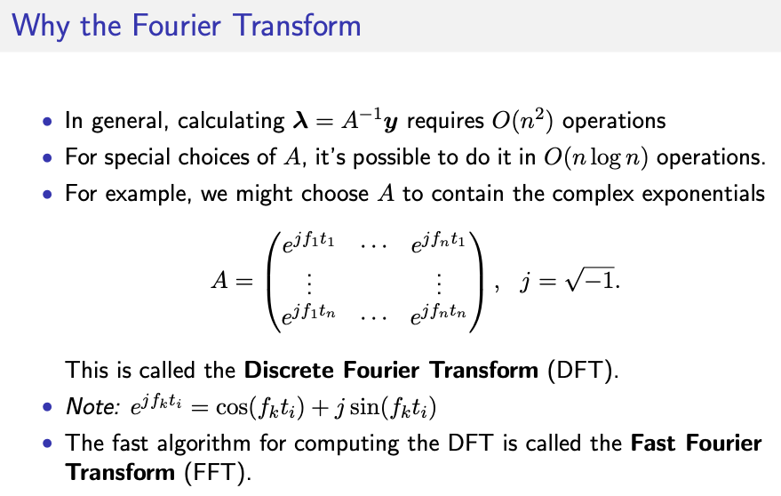
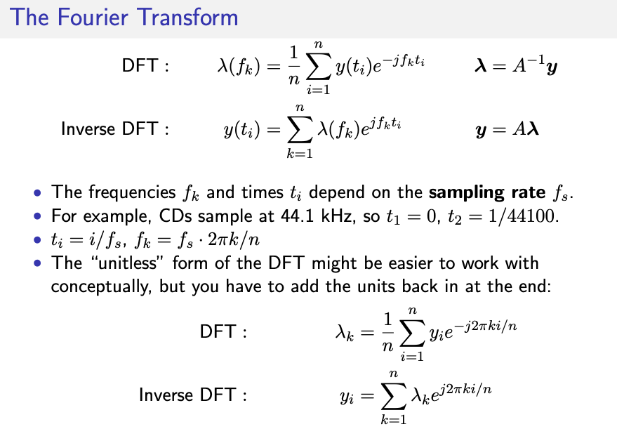
SciTech-Mathmatics-Fourier & Laplace & Spectral Analysis: Sinusoids/Harmonics + FrequenciesSynthesis + Fourier Series: PeriodicalFunctions + (Discrete)FourierTransform:AllFunctions

Laplace Analysis(Fourier Transformation升级版)

注意:
0. "熵增定律": $ \text{衰减函数: } e^{-kt} = e^{ \sigma t} , \ where \ k >0, \ \sigma \ 代\ 衰减度 $

积分域不同: Laplace变换的积分域是 [0, +∞), 而Fourier变换的积分域是 [-∞, +∞]
数域不同: Laplace变换是Complex(复数域)上的，而Fourier变换是Real(实数域)上的。
Laplace变换:

	Equation
Fourier	\(\large \begin{array}{ll} \\ x(t) &= \int_{n=-\infty}^{+\infty}{S_n \cdot e^{ i\omega t}} dt \\ &= \int_{n=-\infty}^{+\infty}{S_n \cdot e^{i(\frac{2\pi n}{T}) t }} dt \\ where, & \\ & \omega \ 代\ Freq.(频率) \\ \end{array}\)
Laplace	\(\large \begin{array}{ll} \\ x(t) &= \int_{n=0}^{+\infty}{S_n \cdot e^{ c t}} dt , \ where \ c \in C(Complex) \\ &= \int_{n=0}^{+\infty}{S_n \cdot e^{ (\sigma + i\omega) t}} dt , \ where \ \sigma = -k,\ k>0 \\ &= \int_{n=0}^{+\infty}{S_n \cdot e^{-kt} \cdot e^{i(\frac{2\pi n}{T}) t }} dt, \ where \ k > 0 \\ where, & \\ & \omega \ 代\ Freq.(频率), \\ & \sigma \ 代\ 衰减度, \ 衰减函数:\ e^{ \sigma t} = e^{-kt}, \ where \ k >0 \\ \end{array}\)

Equation

Fourier

$\large \begin{array}{ll} \\ x(t) &= \int_{n=-\infty}^{+\infty}{S_n \cdot e^{ i\omega t}} dt \\ &= \int_{n=-\infty}^{+\infty}{S_n \cdot e^{i(\frac{2\pi n}{T}) t }} dt \\ where, & \\ & \omega \ 代\ Freq.(频率) \\ \end{array}$

Laplace

$\large \begin{array}{ll} \\ x(t) &= \int_{n=0}^{+\infty}{S_n \cdot e^{ c t}} dt , \ where \ c \in C(Complex) \\ &= \int_{n=0}^{+\infty}{S_n \cdot e^{ (\sigma + i\omega) t}} dt , \ where \ \sigma = -k,\ k>0 \\ &= \int_{n=0}^{+\infty}{S_n \cdot e^{-kt} \cdot e^{i(\frac{2\pi n}{T}) t }} dt, \ where \ k > 0 \\ where, & \\ & \omega \ 代\ Freq.(频率), \\ & \sigma \ 代\ 衰减度, \ 衰减函数:\ e^{ \sigma t} = e^{-kt}, \ where \ k >0 \\ \end{array}$

$\large \begin{array}{ll} \\ S_n &= \frac{1}{T} \int_{t_0}^{t_0+T}{ x(t) \cdot e^{-i\frac{2\pi n t}{T}}} dt \\ & S_n: 分解到正交基函数(复函数)\ e^{i 2\pi n f t}\ 坐标轴上的坐标 \\ \\ \end{array}$

几何角度理解Fourier Series(傅立叶级数)

几何角度看，Fourier Series(傅立叶级数) 其实非常容易理解
0. 每一组$(\cos(2\pi n f t),\ \sin(2\pi n f t))$三角函数都可看作决定一“谐波空间”的 $x$ 轴与 $y$ 轴;
Time-domain 的信号, 是用 Freq.-domain 的 N 个独立空间的谐波合成;
每一个“谐波空间”, 都是一对可配置$( freq.,\ magnitude,\ phase)$的三角函数(cos/sin);
每一个“谐波空间”, 都有三个坐标轴: $(1, \cos(2\pi n f t), \sin(2\pi n f t))$:
$\large \begin{array}{ll} \\ x(t) &= \frac{a_0}{2} + \sum_{n=1}^{\infty} {[\ a_{n} \cos(2\pi n f t) + b_{n}\sin(2\pi n f t) \ ]} \\ & \frac{a_0}{2} \longrightarrow 分解到基函数1(常数函数)对应的坐标轴上的坐标 \\ & a_n \longrightarrow 分解到基函数 \cos(2\pi n f t) 对应的坐标轴上的坐标 \\ & b_n \longrightarrow 分解到基函数 \sin(2\pi n f t) 对应的坐标轴上的坐标 \\ \end{array}$

$\large \begin{array}{ll} \\ x(t) &= \int_{n=-\infty}^{+\infty}{S_n \cdot e^{i\frac{2\pi n t}{T}}} dt \\ S_n &= \frac{1}{T} \int_{t_0}^{t_0+T}{ x(t) \cdot e^{-i\frac{2\pi n t}{T}}} dt \\ & S_n: 分解到正交基函数(复函数)\ e^{i 2\pi n f t}\ 坐标轴上的坐标 \\ \\ \end{array}$

$\large \begin{array}{ll} \\ \\ when & T \rightarrow \infty, \bf{即频域谐波组频点无穷多, 就变成“连续的频带”} \\ F(\omega) &= \frac{1}{2\pi} \int_{-\infty}^{+\infty}{x(t) \cdot e^{-i \omega t}} dt \\ & \omega: 代表频率 \\ \\ \end{array}$

合成的 $\large X(t)$ 周期为 $T = \frac{1}{f}$,
是因为其 $k$ 个Frequency Components(频率成分) 的周期的最小公倍数为 T;
这些 Harmonics(Frequency Components) 谐波任意“加减”组合, 周期最小公倍数为 T.
下文 “Preliminaries.3. Frequency Components) for Synthesis” 有述;
内积(inner product of vectors) 与分解;
- 向量的内积, 在有限维向量空间, 两个向量的内积:
  $\large \begin{array}{rl} \overrightarrow{u} \cdot \overrightarrow{v} &= x_1 x_2 + y_1 y_2 \\ where & \overrightarrow{u} = (x_1, y_1),\ \overrightarrow{v} = (x_2, y_2) \\ \end{array}$
- 函数的内积, 在无限维函数空间, 两个函数(连续)的内积(内积要重新定义,用到积分):
  $\large \begin{array}{rl} <f, g> &= \int_{t_0}^{t_0 + T}{f(t)g(t)} dt \end{array}$
- 离散向量分解:
  将向量 $\overrightarrow{u}$ 分解到两个"正交向量" $\overrightarrow{v_1}$ 与 $\overrightarrow{v_2}$上:
  假设在($\overrightarrow{v_1}$, $\overrightarrow{v_2}$)两坐标轴上坐标为($c_1$, $c_2$), 则有:
  $\large \begin{array}{ll} \ & \\ & \overrightarrow{u} = c_1 \overrightarrow{v_1} + c_2 \overrightarrow{v_2} \\ & 分解出的坐标(c_1, c_2)分别为: \\ & c_1 = \frac{\overrightarrow{u} \cdot \overrightarrow{v_1}}{\overrightarrow{v_1} \cdot \overrightarrow{v_1}},\ c_2 = \frac{\overrightarrow{u} \cdot \overrightarrow{v_2}}{\overrightarrow{v_2} \cdot \overrightarrow{v_2}} \\ \\ \end{array}$
- 连续向量分解:
  将连续向量函数 $\overrightarrow{x(t)}$ 分解到两个"正交基函数" $\overrightarrow{\cos(2\pi n f t)}$ 与 $\overrightarrow{\sin(2\pi n f t)}$上:
  要将以上向量分解公式,由 有限维的向量空间 扩展到 无限维的函数空间;
  要将内积由 有限维的向量空间 扩展到 无限维的函数空间,
  并且, 要将每个三角函数(cos/sin)都看作一个“独立的坐标轴”,
  用到上文的 “函数的内积” 积分公式.
  但是为方便高效, 最好用 $Euler's\ Equation$ 将$cos/sin转换为:
  $\large \begin{array}{ll} \because & s_n &= \frac{1}{T} \int_{t_0}^{t_0 + T}{x(t) \cdot e^{-i2\pi n f t}} dt \\ & T &= \infty \\ \therefore & F(\omega) &= \frac{1}{2\pi} \int_{-\infty}^{+\infty}{x(t) \cdot e^{-i \omega t}} dt \\ \\ \end{array}$
向量的正交与分解: 投影到正交的一堆向量为基的空间;
之所以选择分解到 $f(\theta) = \cos \theta$ 与 $f(\theta) = \sin \theta$, 是因为这是“一对正交基函数”,
而且在任意时刻 $t_0$ 开始, 时长 $2\pi$ 的 $\sin{x} \cos{x}$ 信号的积分都是$0$:
$\large \begin{array}{rl} <sin, cos> &= \int_{ t_0}^{t_0 + 2\pi}{\sin{x} \cos{x}} dx = 0 \end{array}$

类比: 就像$XOY$平面的$X轴$ 与 $Y轴$ 是正交的,
因此$XOY$平面上任何一点, 可用其分别在$X轴$ 与 $Y轴$上的投影作为(x,y)坐标;

向量正交: 对于 $XOY$平面上两个向量 $\overrightarrow{u} = (x_1, y_1),\ \overrightarrow{v} = (x_2, y_2)$,
如果它们的内积为0, 夹角为$90^{\circ}$, 则称这两个向量点是“正交的”, 即 :
$\large \begin{array}{rl} \overrightarrow{u} \cdot \overrightarrow{v} = x_1 x_2 + y_1 y_2 = 0 \\ \end{array}$

函数正交: 余弦函数$ \cos \theta $ 与正弦函数$ \sin \theta $,
可看作 无限维的 Hilbert 空间 的 无限维向量, 向量的各个“元”是连续区间的“函数值”;
无限维空间的向量内积需要用到积分重新定义为“两个连续函数的函数值先相乘后积分”:
$\large \begin{array}{rl} <f, g> &= \int_{x_0}^{x_0 + T}{f(x)g(x)} dx \\ <sin, cos> &= \int_{t_0}^{t_0 + 2\pi}{\sin{t} \cos{t}} dt = 0 \end{array}$
分解 Time-domain 信号到 Frequency-domain,
总体思路上, 与“Taylor Series(泰勒级数)拟合任意N阶可导函数”类似:
- Taylor Series 是以无限项 $\large a_j (x-x_0)^j $(带可调参数的幂函数) 合成任意的 $\large f(x)$;
  确定系数 $\large a_j$ 与 $\large x_0$ 是用 $\large f'(x),\ f''(x), f^{3}(x),\ ...\ ,\ , f^{n}(x)$ 无限高阶导数进行拟合与误差估计;
- Fourier Series 是以无限项 $\large [\ a_{n} \cos(2\pi n f t) + b_{n}\sin(2\pi n f t) \ ]$(可配置系数的sin正弦信号发生器);
  确定系数 $a_n$ 与 $b_n$ 是用积分/复数运算进行拟合与误差估计;
实际上, 把 Time-domain 的 Signal 函数 $X(t)$ 分解/投影到 Frequency-domain 的多个“平面”(sin信号发生器):
- 每个“平面”有一对“正交基函数”(cos/sin), 实现上是一组($N$个)“可配置系数”的sin信号发生器(谐波信号轮);
  每个“sin正弦信号轮”的用:
  - 半径(Radius)表示$magnitude$系数,
  - 用起始的距0弧度的bias量表示$phase$系数,
  - 以配置的常数的转动频率周期转动(产生信号)表示 Harmonic($\large nf_0$) 固定的谐波频率;
  通过这一组($N$个)“sin信号轮”以配置好的$(magnitude,\ phase,\ harmonic)$同时转动(产生信号),
  可以合成任意的周期函数; 谐波信号轮个数越多($N$越大)越精准;
- 参数 $(a_j, b_j)$ 可以导出$(magnitude,\ phase)$, 因为 $frequency$这个系数,
  总是 Harmonic(谐波频点, “基频$\large f$”的自然数倍), 所以可视为可变的常数;
  因此实际最需要确定的系数$(magnitude,\ phase)$用 $(a_j, b_j)$ 导出就足够;
  Sampling在任意时刻$\large t_0$, 最短采集($\bf{T_0 = \frac{1}{f_0}}$(the fundamental period)$时长就足够;
既可以选用 sin 系列的正弦函数, 也可以选用 cos系列的余弦函数;
之所以选用 cos 与 sin 两个函数作为“基函数”:
- 因为 cos 与 sin 这一对“基函数”正交.
- cos 与 sin 可以非常好的与 Complex Space 转换;
- cos 与 sin 可以用 Euler's Equation $\large e^{i\theta} = \cos\theta + i \sin\theta $ 进行变换计算;
- cos 与 sin 在实现、转换、变换以及实际应用时非常方便实现.
  $\large cos\theta$ 可用 $\large sin{(\theta - \frac{\pi}{2})}$ 合成(即phase左移$\large \frac{\pi}{2}$);
  实现上, 只要做好一种可配置(freq., magnitude, phase)的 sin正弦信号发生器就可规模化量产;
- 总之优点众多.

Fourier Analysis Preliminaries

Periodic signals:

At least to begin, we’ll mainly be concerned with signals that are periodic.
Informally, a periodic signal is one that repeats, over and over, forever. To be more precise:
A signal $x(t)$ is said to be periodic if there exists some number $T$,
$\large \begin{array}{lll} \text{such that} & \\ x(t) &=& x(t+T) \text{ , for all } t \\ & & \ T:\ \mathbf{\text{the period of the signal} } \\ & & \ \mathbf{smallest\ } T:\ \mathbf{\text{the fundamental period}} \\ \end{array}$.
Sinusoids:

Precisely what do we mean by a sinusoid? The term “sinusoid” means a sine wave,
but we don’t just mean the standard $\sin(t)$. To enable our analysis,
we want to be able to work sine waves of different $heights$, $widths$ and $phases$.
So, to us, a single sinusoid means a function of the form
$\large \begin{array}{lll} \\ \ \ \ \ & x(t) &= A& \sin(2\pi f t + \phi) \\ \text{for some} & & \\ & & A &its\ amplitude \\ & & f &its\ frequency,\ period\ T = \frac{1}{f} \\ & & \phi &its\ phase \\ \end{array}$,
Frequency Components for Synthesis:

$\begin{array}{rlll} GIVING& &&& \\ x_{1}(t) &=& A_1 \sin (1 \times (2\pi f t + \phi ) ) \ ,\ \text{ freq.: } \ f\ ,\ \text{ amplitude:} A_1\ ,\ \text{ phase:} \ \phi \\ x_{2}(t) &=& A_2 \sin (2 \times (2\pi f t + \phi) ) \ ,\ \text{ freq.: } 2f\ ,\ \text{ amplitude:} A_2\ ,\ \text{ phase:} 2\phi \\ x_{3}(t) &=& A_3 \sin (3 \times (2\pi f t + \phi) ) \ ,\ \text{ freq.: } 3f\ ,\ \text{ amplitude:} A_3\ ,\ \text{ phase:} 3\phi \\ ...& & \\ x_{k}(t) &=& A_k \sin (k \times (2\pi f t + \phi) ) \ ,\ \text{ freq.: } nf\ ,\ \text{ amplitude:} A_k\ ,\ \text{ phase:} k\phi \\ \\ X(t) &=& \sum_{n=1}^{k} x_{n}(t) & \\ &=& \sum_{n=1}^{k} { A_{n} \sin[\ n(2\pi f t + \phi)\ ] } & \\ \\ \end{array}$
$\text{ THEN the }\mathbf{period}\ of\ X(t)\text{ is } T = \frac{1}{f}, \text{SINCE}$
$\begin{array}{rlll} \\ \ \ period(x_{1}) &= T &= \frac{1}{f}, \\ \ \ period(x_{2}) &= \frac{T}{2} &= \frac{1}{2f}, \\ \ \ period(x_{3}) &= \frac{T}{3} &= \frac{1}{3f}, \\ \ \ &... & \\ \ \ period(x_{k}) &= \frac{T}{k} &= \frac{1}{kf}, \\ \\ \end{array}$
Harmonics/Sinusoids:

The sinusoidal terms are often called $\mathbf{harmonics}$, a term borrowed from music.
The harmonics will have frequencies $f\ ,\ 2f\ ,\ 3f\ ,\ 4f$ and so on.
We also call each $harmonic$, $A_n \sin(2\pi n f t + \phi n)$, the $\mathbf{frequency\ component}$ of $x(t)$ at frequency $n f$.
For example, if $f = 10Hz$, we call the $harmonic$ for which
$n = 3$ the “$30Hz\ component$”, reflecting that
in this case $\sin(2\pi n f t+\phi n)$ is a sinusoid of frequency $30Hz$
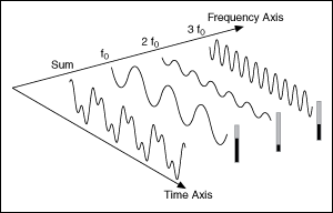
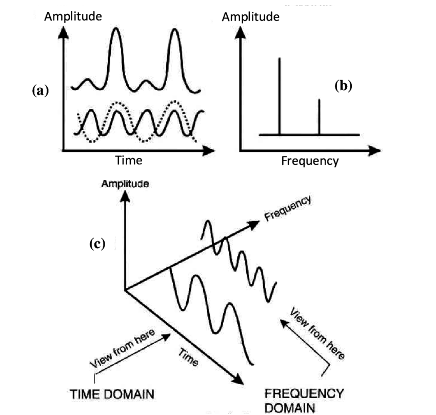
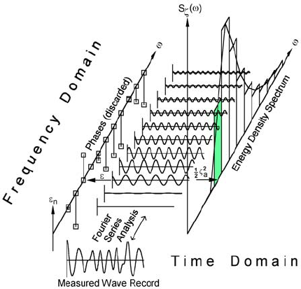
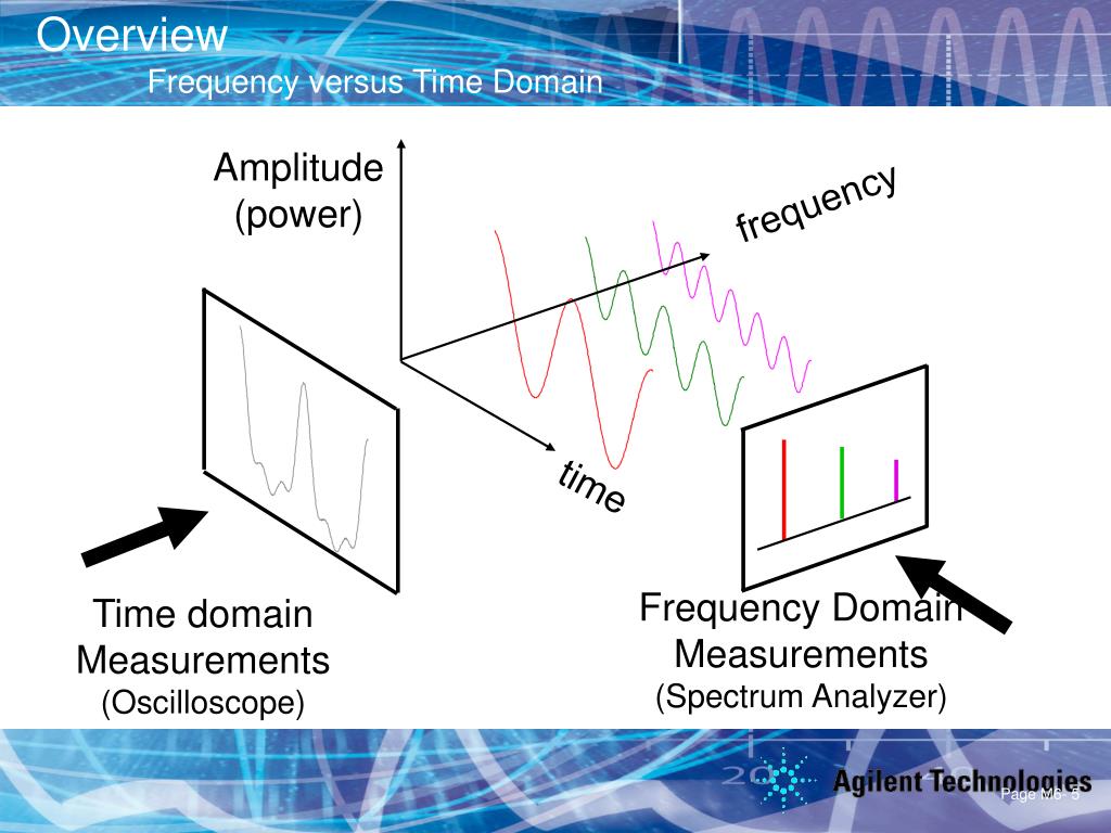
Frequency-domain and Time-domain Representation:
- the frequency-domain representation of the periodic signal:
  represent a signal using the magnitudes and phases in its Fourier series.
  We often plot the magnitudes in the Fourier series,
  using a stem graph and labeling the frequency axis by frequency.
  In this sense, this representation is a function of frequency.
- the time-domain representation of the signal:
  represent a periodic signal as a function of time in its Fourier series.
- Example:

The Fourier Series:

Joseph Fourier’s idea was to express periodic signals as a sum of sinusoids.
Theorem.
- If $\mathbf{ x(t) }$ is a $\text{ well-behaved periodic signal }$ with $\large \mathbf{ period\ T}$,
  
  $\large \text{ We call }\mathbf{\ following\ sum } \ the\ \mathbf{\ Fourier\ series\ of\ }x(t) $
  $\large \begin{array}{ll} x(t) &= \begin{equation} A_0 + \sum_{n=1}^{\infty} { A_{n} \sin(2\pi n f t + n\phi) } \tag{1F} \end{equation} \\ & \mathbf{ frequency }: f = 1/T, \\ & \mathbf{ magnitudes }: A_i\ ,\ i \in [\ 1, +\infty\ ] \\ & \mathbf{ phases } \phi_i\ ,\ i \in [\ 1, +\infty\ ] \\ \\ \end{array}$
  Another fact relating to Fourier series is that:
  the $magnitudes\ A_0\ ,\ A_1\ ,\ A_2\ ,\ ... $ and $phases\ \phi_1\ ,\ \phi_2\ ,\ ... $
  in above equation uniquely determine $x(t)$. That is, if we can find these
  $ magnitudes $ and $phases$ corresponding to a periodic signal $x(t)$,
  then, in effect, we have another way of describing $x(t)$.
- $\large \text{ Another useful form of Fourier series of }x(t)$
  $\large \begin{array}{ll} x(t) &= \begin{equation} \frac{a_0}{2} + \sum_{n=1}^{\infty} {[\ a_{n} \cos(2\pi n f t) + b_{n}\sin(2\pi n f t) \ ]} \tag{2F} \end{equation} \\ & a_{0} = 2 A_0\ , \\ & a_{n} = A_{n}\cos{(n\phi)}\ ,\ b_{n} = A_{n}\sin{(n\phi)}\ , \\ & (a_{n})^{2} + (b_{n})^{2} = (A_{n})^{2}\ \\ & \text{ above } \mathbf{coefficients}\text{ can then be found, } \\ & \text{ using the following integrals, where }T = \frac{1}{f}: \\ & a_n = \frac{2}{T} \int_{0}^{T}{x(t)\cos(2\pi n f t)} dt \, \\ & b_n = \frac{2}{T} \int_{0}^{T}{x(t)\sin(2\pi n f t)} dt \\ &\text{ and }a_0,\ a_1,\ a_2,\ . . .\text{ and }b_1,\ b_2,\ . . .\ \\ &\text{ can be converted to }magnitudes\text{ and }phases,\ \\ &\text{ to fit above form (1F) }. \\ \\ \end{array}$
  
  $\large \text{ Proof of form (1F) and form (2F) are the same }$
  $\large \begin{array}{lll} \\ & \because & \sin(X + Y) = \sin{X} \cos{Y} + \cos{X} sin{Y} \\ & \therefore & \sin(2\pi n f t + n\phi) = \sin{(2\pi n f t)} \cos{(n\phi)} + \cos{(2\pi n f t)} sin{(n\phi)} \\ & x(t) &= A_0 + \sum_{n=1}^{\infty} { A_{n} \sin(2\pi n f t + n\phi) } \\ & &= A_0 + \sum_{n=1}^{\infty} { (A_{n}\cos{(n\phi)}) \sin{(2\pi n f t)} + (A_{n}\sin{(n\phi)}) \cos{(2\pi n f t)}\ ] } \\ & & = \frac{a_0}{2} + \sum_{n=1}^{\infty} {[\ a_{n} \cos(2\pi n f t) + b_{n}\sin(2\pi n f t) \ ]} \\ \\ \end{array}$
- $\large \text{ Complex form of Fourier series of }x(t)$
  $\large \begin{array}{lll} \because e^{i\theta} &= \cos\theta + i\sin\theta ,\text{ the Euler's Equation}\\ \therefore e^{i2 \pi n f t} &= \cos{(2 \pi n f t)} + i\sin{(2 \pi n f t)} \\ x(t) &= \frac{a_0}{2} + \sum_{n=1}^{\infty} {[\ a_{n} \cos(2\pi n f t) + b_{n}\sin(2\pi n f t) \ ]} \\ &= \frac{1}{T} \int_{t_0}^{t_0 + T}{x(t) \cdot e^{-i2\pi n f t}} dt \\ \\ \end{array}$
  
  $\large \begin{array}{ll} \because & S_n &= \frac{1}{T} \int_{t_0}^{t_0 + T}{x(t) \cdot e^{-i2\pi n f t}} dt \\ & T &= \infty \\ \therefore & F(\omega) &= \frac{1}{2\pi} \int_{-\infty}^{+\infty}{x(t) \cdot e^{-i \omega t}} dt \\ \\ \end{array}$

Time Domain + Frequency Domain

and Fourier Transforms @ Princeton University:

Fourier Series: Periodical Functions

Fourier Transform: All Functions
Frequency Domain and Fourier Transforms @ Princeton University:
https://www.princeton.edu/~cuff/ele201/kulkarni_text/frequency.pdf

Signals and the frequency domain

ENGR 40M lecture notes — July 31, 2017 Chuan-Zheng Lee, Stanford University
https://web.stanford.edu/class/archive/engr/engr40m.1178/slides/signals.pdf

https://www.mathworks.com/help/signal/ug/extract-regions-of-interest-from-whale-song.html

https://web.stanford.edu/class/stats253/lectures_2014/lect7.pdf
https://web.stanford.edu/class/stats253/lectures_2014/
https://resources.pcb.cadence.com/blog/2020-time-domain-analysis-vs-frequency-domain-analysis-a-guide-and-comparison

Time Domain and Frequency Domain:
- Illustrations:
  | | | |
  | ---- | ---- | ---- |
  | | | |

Application: The role of ECoG magnitude and phase in decoding position, velocity, and acceleration during continuous motor behavior

Frequency Domain and Fourier Transforms @ Princeton University:
https://www.princeton.edu/~cuff/ele201/kulkarni_text/frequency.pdf
Signals @ WEB.stanford.edu
https://web.stanford.edu/class/archive/engr/engr40m.1178/slides/signals.pdf
https://web.stanford.edu/class/stats253/lectures_2014/lect7.pdf

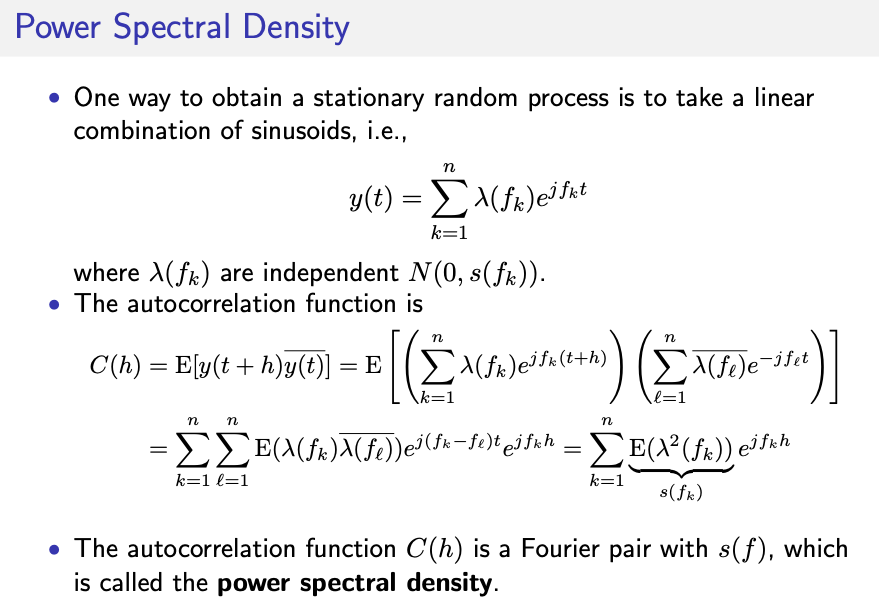
The Frequency Domain

(Discrete) Fourier Transform

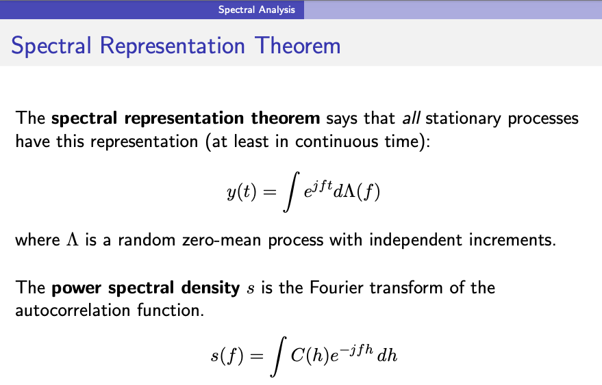
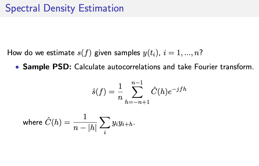
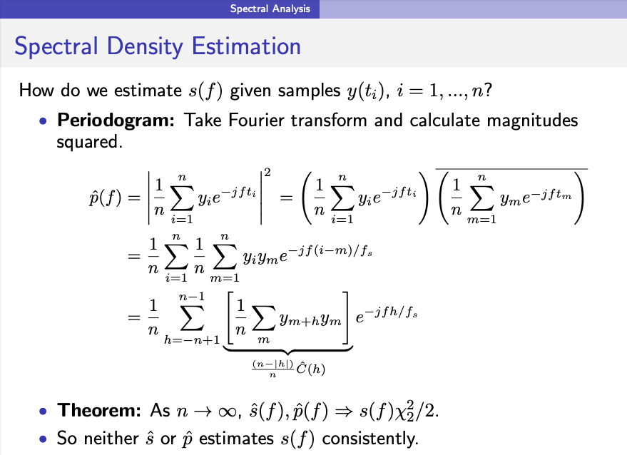
Spectral Analysis

This is a new course.
• The material that we will be covering has not really been synthesized—because it is at the frontiers of statistics!
• We will be loosely following the books
• Shumway and Stoffer. Time Series Analysis and Applications (with R
Applications).
• Sherman. Spatial Statistics and Spatio-Temporal Data.
• You don’t have to purchase these books: they are available for free for Stanford students. (Link on course website.)
• Other useful references:
• Bivand et al. Applied Spatial Data Analysis with R. (also available free) • Cressie and Wikle. Statistics for Spatio-Temporal Data.