IIR数字滤波器设计

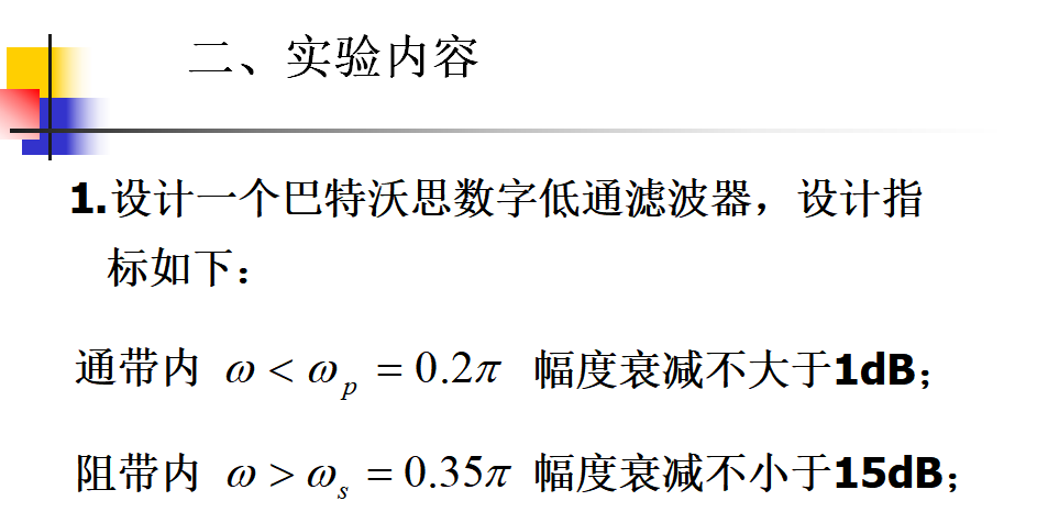
%实验三(1)  设计要求的数字滤波器
clc;clear;
clear all;
wp=0.2;ws=0.35;Ap=1;As=15;     
[N,fc]=buttord(wp,ws,Ap,As);    %求出符合参数的滤波器阶数和截止频率
[B,A]=butter(N,fc);             %得到滤波器H(z)的系数
[h,w]=freqz(B,A,1024);          %计算模拟滤波器响应
plot(w/pi,20*log10(abs(h)/abs(h(1))));
title('wp=0.2π;ws=0.35π;Ap=1dB;As=15dB的巴特沃思数字低通滤波器');
grid on;xlabel('w/pi');ylabel('幅度(dB)');
axis([0,1,-30,0])
line([0,1],[-1,-1],'linestyle','--');
line([0,1],[-15,-15],'linestyle','--');
line([0.2,0.2],[-30,0],'linestyle','--');
line([0.35,0.35],[-30,0],'linestyle','--');

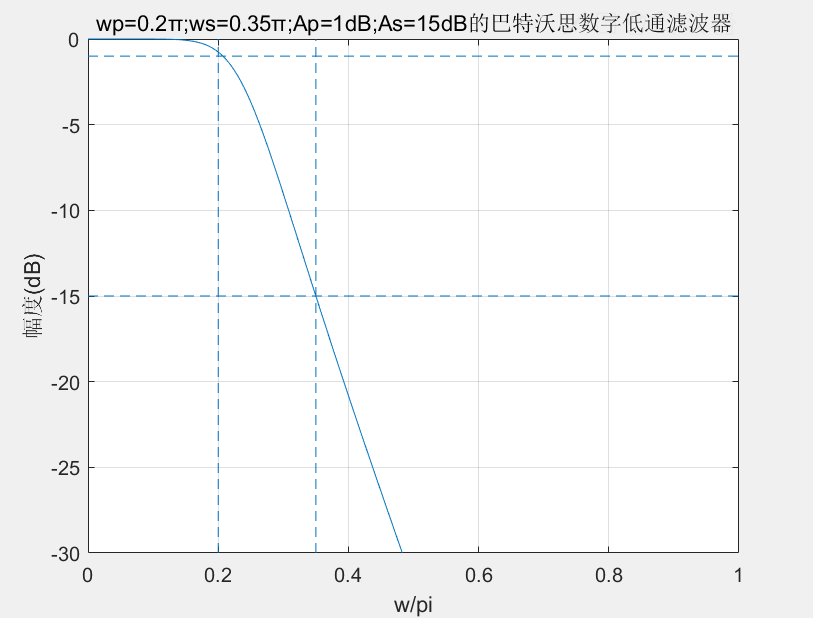
编制计算设计的数字滤波器幅度特性和相位特 性的程序，并进行实验验证。

%实验三(2)  数字滤波器的幅度特性与相位特性
clc;
close all;
wp=0.2;ws=0.35;Ap=1;As=15;
[N,fc]=buttord(wp,ws,Ap,As);     %求出符合参数的巴特沃思滤波器阶数和截止频率
[b,a]=butter(N,fc);              %得到滤波器H(z)的系数
[h,w]=freqz(b,a,1024);           %计算数字滤波器响应
subplot(2,1,1);plot(w/pi,abs(h));title('幅度响应');     %数字滤波器幅度特性
axis([0,1,0,1.2]);line([0.2,0.2],[0,1.2],'linestyle','--');
line([0.35,0.35],[0,1.2],'linestyle','--');
xlabel('w/pi');ylabel('幅度');
subplot(2,1,2);plot(w/pi,angle(h)/pi);title('相位响应'); %数字滤波器相频特性
axis([0,1,-1,1]);line([0.2,0.2],[-1,1],'linestyle','--');
line([0.35,0.35],[-1,1],'linestyle','--');
xlabel('w/pi');ylabel('相位/pi');

 编制实现该数字滤波器程序并且实现数字滤波

%实验三(3)  实现各个频率的正弦波的数字滤波
clc; clear;
close all;
wp=0.2;ws=0.35;Ap=1;As=15;
[N,fc]=buttord(wp,ws,Ap,As);     %求出符合参数的巴特沃思滤波器阶数和截止频率
[b,a]=butter(N,fc);              %得到滤波器H(z)的系数
[H,w]=freqz(b,a,1024);           %计算数字滤波器响应
[h,n]=impz(b,a,30);
w1=0.15*pi;w2=0.3*pi;w3=0.4*pi;
x1=sin(w1.*n);x2=sin(w2.*n);x3=sin(w3.*n); %正弦波频率:通带、过渡带、阻带
figure
subplot(3,2,1);   stem(n,x1); title('通带正弦波'); %原通带正弦波
subplot(3,2,2);   y1=conv(x1,h); stem(0:length(y1)-1,y1);axis([0,60,-1,1]); title('滤波后的通带正弦波'); 
subplot(3,2,3);   stem(n,x2); title('过渡带正弦波'); %原过渡带正弦波   
subplot(3,2,4);   y2=conv(x2,h); stem(0:length(y2)-1,y2);axis([0,60,-1,1]); title('滤波后的过渡带正弦波'); 
subplot(3,2,5);   stem(n,x3); title('阻带正弦波');  %原阻带正弦波
subplot(3,2,6);   y3=conv(x3,h); stem(0:length(y3)-1,y3);axis([0,60,-1,1]); title('滤波后的阻带正弦波'); 
figure      
w4=0.6*pi;x4=sin(w4.*n);  %验证滤波器的模拟截止频率，滤波后的幅度几乎全0
subplot(2,1,1);   stem(n,x4); title('截止频率处的正弦波'); 
subplot(2,1,2);   y4=conv(x4,h); stem(0:length(y4)-1,y4);axis([0,60,-1,1]); title('滤波后的正弦波'); 

 

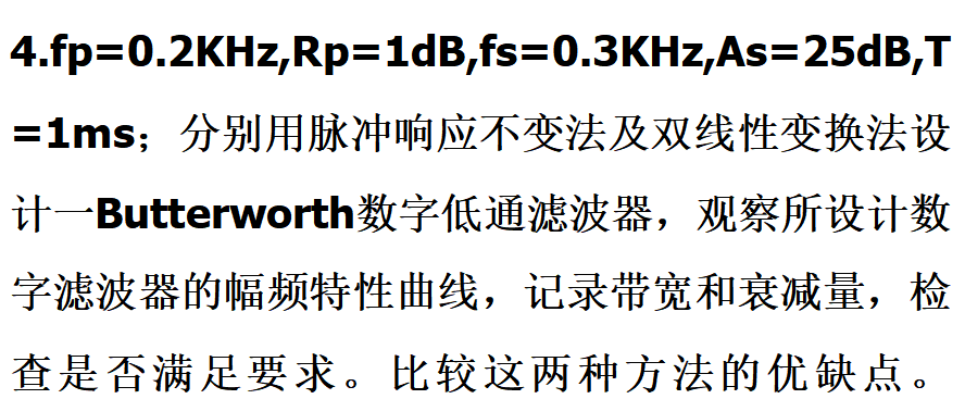
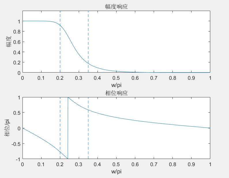
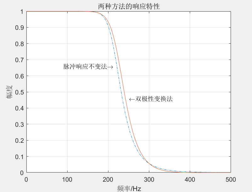
%实验三(4)      冲激响应不变法与双极性变换法的对比
clc;
close all;
fp=200;fs=300;Rp=1;As=25;T=0.001;
%使用脉冲响应不变法（存在频率混叠）
wp=2*pi*fp*T;ws=2*pi*fs*T;  %wp、ws为数字频率
Wp=wp/T;Ws=ws/T;            %Wp、Ws为模拟频率
[N1,fc]=buttord(Wp,Ws,Rp,As,'s');
[b,a]=butter(N1,fc,'s');
[b1,a1]=impinvar(b,a,1/T);   %冲击响应不变法变换到数字滤波器
[h1,w]=freqz(b1,a1);
%使用双极性变换法（不存在频率混叠）
Wp=2/T*tan(wp/2);Ws=2/T*tan(ws/2);  %频率预畸变
[N1,fc]=buttord(Wp,Ws,Rp,As,'s');   
[b,a]=butter(N1,fc,'s');
[b2,a2]=bilinear(b,a,1/T);   %双极性变换法变换到数字滤波器
[h2,w]=freqz(b2,a2);
f=w/2/pi/T;
figure
plot(f,abs(h1),'-.',f,abs(h2),'-');
text(90,0.66,'脉冲响应不变法\rightarrow');
text(250,0.46,'\leftarrow双极性变换法');
axis([0,500,0,1]);grid on;
xlabel('频率/Hz');ylabel('幅度');