关于正则化
Everything you need to know about Regularization
Different ways to prevent over-fitting in machine learning
If you're working with machine learning models, you've probably heard of regularization. But do you know what it is and how it works? Rgularization is a technique used to prevent overfitting and improve the perfromance of models. In this post, we'll break down the different types of regularization and how you can use them to improve your models. Besides, you learn when to apply the different types.
Regularization in machine learning means 'simplifying the outcome'. In case a model is over-fitting and too complex, you can use regularization to make the model generalize better. You should use regularization if the gap in performance between train and test is big. This means the model grasps too much details of the train set. Over-fitting is related to high variance, which means the model is sensitive to specific samples of the train set.
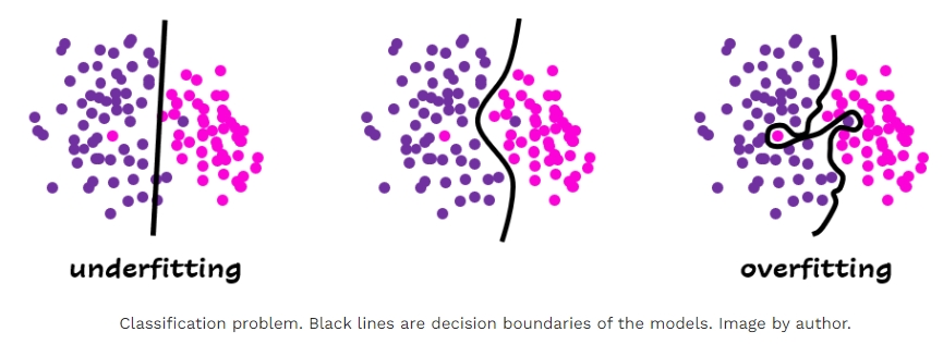
Especially, when performing a machine learning task on a small dataset, one often suffers from the over-fitting problem, where the model accurately remembers all training data, including noise and unrelated features. Such a model often performs badly on new test or real data that have not been seen before. Because the model treats the training data too seriously, it failed to learn any meaningful pattern out it, but simply memrorizing everything it has seen.
Over-fitting means that the model is too "smart" and thinks too much, so that it loses the ability to generalize. Regularization bangs on your model to make it "dumber". So instead of simply memorizing stuff, it has to look for simplier patterns from the data.
All techniques that fall into explicit regularization are explicitly adding a term to the problem. We will dive into the three most common types of explicit regularization. These types are \(\ell_{1}\), \(\ell_{2}\) and Elastic Net regularization.
A most common form of this type of problems
where \(A\in\mathbb{R}^{n\times d}\). In the field of machine learning, \(A\) is a matrix that constains all the training data, \(x\) is the solution vector you are looking for, \(y\) is the label vector.
It is also the ordinary least squares (OLS) problem.
\(\ell_{1}\) regularization
Motivation: Sparse models
While computing a model to explain some data, we might want to compute a model that expalins the data using as few feature as possible. Mathematically speaking, if our model is parameterized by a vector \(x\in\mathbb{R}^{d}\), our goal is to compute a vector that explains the data with as few nonzeros coordinates as possible.
There exists a regularizer that penalized vectors with nonzero components, called the \(\ell_{0}\) norm (though thchnically this function defines a semi-norm). An \(\ell_{0}\)-regularized problem has form
where \(\lambda>0\) is a regularization parameter. Nevertheless, theis function is nonsmooth and discontinuous; its combinatorial nature also introduces more complexity to the original problem.
As a result, researchers have turned to an intermediate regularization term, the \(\ell_{1}\) norm defined by
This function is continuous and convex; moreover, it is a norm function, which endows it with many desirable properties. As a result, the class of problems of the form
called \(\ell_{1}\) regularized problems or lasso problems, has emerges as a tractable alternative to the \(\ell_{0}\) regularized formulation.
By \(\ell_{1}\) regularization, you essentially make the vector \(x\) smaller (sparse), as most of its components are useless (zeros), and at the same time, the remaining non-zero components are very "useful".
A natural way to tackle problems of the above form is through the \(\color{blue}{proximal \ gradient}\) framework. Indeed, unlike for general regularizers, one can obtain a closed-form solution, the proximal subproblem, given by
has a unique solution. To obtain it, one computes the usual step \(x_{k}-\alpha_{k}\nabla f(x_k)\), then one applies the \(\color{blue}{soft-thresholding \ function}\) \(s_{\alpha_{k}\lambda}(+)\) to each component, where this function is given by
(Note that this function encodes the proximal operator for the \(\ell_{1}\) norm.) As a result, the solution of the proximal subproblem is defined component-wise according to the components of the garadientstep. The resulting update is at the heart of the corresponding proximal algorithm, popularized in signal and image processing under the name ISTA (Iterative Soft-Thresholding Algorithm).
It can be shown that use of the soft-thresholding function does promote zero compnents in the new iterates.
A notable improvement on ISTA was the inclusion of the momentum, which resulted in a new algorithm called FISTA (Fast ISTA): this method is now the most widely used instance of ISTA.
\(\ell_{2}\) regularization
Motivation: Stable models
\(\ell_{2}\) regularization, or Ridge regularization, adds a term to the cost function that is proportional to the square of the weight coefficients. The most common instance of \(\ell_{2}\)-regularized problem is a linear-squares loss is an important class of problems. Such problems have the form
where \(A\in\mathbb{R}^{n\times d}\) and \(y\in\mathbb{R}^{n}\) from the problem data, and \(\lambda>0\).
This term tends to shrink all of the weight coefficients, but unlike \(\ell_{1}\) regularization, it does not set any weight coefficients to zero.
The regularization parameter does not change the nature of the problem, in that it remains a linear least-squares problem. Nevertheless, the above problem is necessarily strongly convex, whereas the un-regularized problem \(\text{minimize}_{x\in\mathbb{R}^{d}}\frac{1}{2}\|Ax-y\|_{2}^{2}\) may not be. As mentioned above, bringing strong convexity is a motivation for using \(\ell_{2}\) regularization.
Suppose that \(d<n\). Then,
a): If \(A^{T}A\) is not invertible, the un-regularized problem has infinitely many solutions.
b): If \(A^{T}A\) is invertible, there exists a unique solution to the un-regularized problem given by
c): For any \(\lambda>0\), the regularized problem has a single solution given by
(Note that the result for the unregularized problem is actually independent of the assumption on \(n\) and \(d\).)
Looking at the formulas for \(\hat{x}\) and \(x^{*}(\lambda)\), we see that \(x^{*}(\lambda)\rightarrow\hat{x}\) as \(\lambda\rightarrow 0\) and \(x^{*}(\lambda)\rightarrow \mathbb{0}_{\mathbb{R}^{d}}\) as \(\lambda\rightarrow\infty\). As \(\lambda\) increases, the importance of \(A\) and \(y\) in the definition of the solution is gradually reduced. In that sense, the solution is less sensitive to changes in the data. Additionally, the regularization leads to a solution with coordinates that are of the same magnitude.
\(\textbf{Example 1}.\) Let \(n=d=2\), \(A=\begin{bmatrix} 1 &0\\ 0 &\epsilon \end{bmatrix}\) for some \(\epsilon>0\) and \(y=\begin{bmatrix}1 \\1 \end{bmatrix}\). Then, we have
whose norm is of order \(\frac{1}{\epsilon}\) for small \(\epsilon\). However, for any \(\lambda>0\), we obtain
whose norm is \(O(\frac{1}{\lambda})\) for \(\lambda\) sufficiently large, regardless of the value of \(\epsilon\). In this sense, regularizing leads to a more stable solution.
Elastic net regularization
This is a combination of both \(\ell_{1}\) and \(\ell_{2}\) regularization. As you would expect, with Elastic Net regularization, both of the \(\ell_{1}\) and \(\ell_{2}\) terms are added to the cost function. And a new hyperparameter α is added to control the balance between \(\ell_{1}\) and \(\ell_{2}\),
When to use \(\ell_{1}\), \(\ell_{2}\) or Elastic Net?
In many scikit-learn models \(\ell_{2}\) is the default (see LogisticRegression and SupportVectorMachines). This is for a reason: \(\ell_{1}\) tends to shrink some of the weight coefficients to zero, which means the features are removed from te model. So \(\ell_{1}\) regularization is more useful for feature selection (Sparsity). To really prevent overfitting, \(\ell_{2}\) might be the better choice, because it does not set any of the weight coefficients to zero.
Elastic Net regularization is a good choice when you have correlated features and you want to balance the feature selection and over-fitting prevention. It's also useful when you're not sure whether \(\ell_{1}\) or \(\ell_{2}\) regularization would be more appropriate for your data and model.
In general, \(\ell_{2}\) regularization is recommended when you have a large number of features and you want to keep most of them in the model, and \(\ell_{1}\) regularization is recommended when you have a high-dimensional dataset with many correlated features and you want to select a subset of them.
Selecting regularization parameter
Last but not least, in the regularized models with different norm penalty, a crucial variable affecting the performance of algorithm is the regularization parameter. How to choose an appropriate regularization parameter is still an open problem.
Now let's consider the parameter selection in the \(\ell_{1}\) regularization model. Review the previous analysis, if we perform machine learning on a small dataset without adding a regularization term, it will lead to a over-fitting phenomenon. Imagine, if the training dataset is large enough and includes all the data in the field (just an idealized assumption), what will happen in this case? My answer is that regularization term is not needed, because on a large enough dataset, the model trained is real.
Aha, it seems that I said nonsense, but it's not the case. On a small dataset, due to incomplete information, increasing the regularization helps to enhance the generalization ability of the model; conversely, on a large dataset, a smaller regularization can prevent over-fitting. The conclusion is that the size of the regularization parameter is inversely proportional to the size of the dataset.

 浙公网安备 33010602011771号