机器学习—分类3-2（朴素贝叶斯算法）

基于朴素贝叶斯预测客户是否购买汽车新车型

主要步骤流程：

• 1. 导入包
• 2. 导入数据集
• 3. 数据预处理
  • 3.1 检测缺失值
  • 3.2 生成自变量和因变量
  • 3.3 查看样本是否均衡
  • 3.4 将数据拆分成训练集和测试集
  • 3.5 特征缩放
• 4. 构建朴素贝叶斯模型做预测
  • 4.1 构建模型并训练
  • 4.2 预测测试集
  • 4.3 生成混淆矩阵
  • 4.4 可视化测试集的预测结果
  • 4.5 评估模型性能

 

 数据集链接：https://www.cnblogs.com/ojbtospark/p/16006391.html

 

1. 导入包

In [1]:

# 导入包
import numpy as np
import pandas as pd
import matplotlib.pyplot as plt

 

2. 导入数据集

In [2]:

# 导入数据集
dataset = pd.read_csv('Social_Network_Ads.csv')
dataset

Out[2]:

	User ID	Gender	Age	EstimatedSalary	Purchased
0	15624510	Male	19	19000	0
1	15810944	Male	35	20000	0
2	15668575	Female	26	43000	0
3	15603246	Female	27	57000	0
4	15804002	Male	19	76000	0
...	...	...	...	...	...
395	15691863	Female	46	41000	1
396	15706071	Male	51	23000	1
397	15654296	Female	50	20000	1
398	15755018	Male	36	33000	0
399	15594041	Female	49	36000	1

400 rows × 5 columns

 

3. 数据预处理

3.1 检测缺失值

In [3]:

# 检测缺失值
null_df = dataset.isnull().sum()
null_df

Out[3]:

User ID            0
Gender             0
Age                0
EstimatedSalary    0
Purchased          0
dtype: int64

3.2 生成自变量和因变量

为了可视化分类效果，仅选取 Age 和 EstimatedSalary 这2个字段作为自变量

In [4]:

# 生成自变量和因变量
X = dataset.iloc[:, [2, 3]].values
y = dataset.iloc[:, 4].values

In [5]:

X[:5, :]

Out[5]:

array([[   19, 19000],
       [   35, 20000],
       [   26, 43000],
       [   27, 57000],
       [   19, 76000]], dtype=int64)

3.3 查看样本是否均衡

In [6]:

# 查看样本是否均衡
sample_0 = sum(dataset['Purchased']==0)
sample_1 = sum(dataset['Purchased']==1)
print('不买车的样本占总样本的%.2f' %(sample_0/(sample_0 + sample_1)))

不买车的样本占总样本的0.64

3.4 将数据拆分成训练集和测试集

In [7]:

# 将数据拆分成训练集和测试集
from sklearn.model_selection import train_test_split
X_train, X_test, y_train, y_test = train_test_split(X, y, test_size = 0.25, random_state = 0)
print(X_train.shape)
print(X_test.shape)
print(y_train.shape)
print(y_test.shape)

(300, 2)
(100, 2)
(300,)
(100,)

3.5 特征缩放

In [8]:

# 特征缩放
from sklearn.preprocessing import StandardScaler
sc = StandardScaler()
X_train = sc.fit_transform(X_train)
X_test = sc.transform(X_test)

 

4. 构建朴素贝叶斯模型做预测

4.1 构建模型并训练

In [9]:

# 构建高斯朴素贝叶斯模型并训练模型
from sklearn.naive_bayes import GaussianNB
classifier = GaussianNB()
classifier.fit(X_train, y_train)

Out[9]:

GaussianNB()

4.2 预测测试集

In [10]:

# 预测测试集
y_pred = classifier.predict(X_test)
y_pred[:5]

Out[10]:

array([0, 0, 0, 0, 0], dtype=int64)

4.3 生成混淆矩阵

In [11]:

# 生成混淆矩阵
from sklearn.metrics import confusion_matrix
cm = confusion_matrix(y_test, y_pred)
print(cm)

[[65  3]
 [ 7 25]]

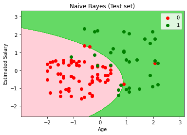
4.4 可视化测试集的预测结果

In [12]:

# 可视化测试集的预测结果
from matplotlib.colors import ListedColormap
plt.figure()
X_set, y_set = X_test, y_test
X1, X2 = np.meshgrid(np.arange(start = X_set[:, 0].min() - 1, stop = X_set[:, 0].max() + 1, step = 0.01),
                     np.arange(start = X_set[:, 1].min() - 1, stop = X_set[:, 1].max() + 1, step = 0.01))
plt.contourf(X1, X2, classifier.predict(np.array([X1.ravel(), X2.ravel()]).T).reshape(X1.shape),
             alpha = 0.75, cmap = ListedColormap(('pink', 'limegreen')))
plt.xlim(X1.min(), X1.max())
plt.ylim(X2.min(), X2.max())
for i, j in enumerate(np.unique(y_set)):
    plt.scatter(X_set[y_set == j, 0], X_set[y_set == j, 1],
                color = ListedColormap(('red', 'green'))(i), label = j)
plt.title('Naive Bayes (Test set)')
plt.xlabel('Age')
plt.ylabel('Estimated Salary')
plt.legend()
plt.show()

4.5 评估模型性能

In [13]:

# 评估模型性能
from sklearn.metrics import accuracy_score
print(accuracy_score(y_test, y_pred))

0.9

In [14]:

(cm[0][0] + cm[1][1])/(cm[0][0] + cm[0][1] + cm[1][0] + cm[1][1])

Out[14]:

0.9

 

结论：1）由上图可见，朴素贝叶斯分类可以做非线性分类。