神经网络--线性神经网络---异或问题---代码示例
‘’‘’‘’
依然是单层神经网络
import numpy as np
import matplotlib.pyplot as plt

'''
在上篇博客中,我们实现了简单单层感知机用来分类,但是异或问题不能被解决

假设我们的数据集依然是x1 ,x2  ,但是我们需要补充更多的输入 x1*x1 ,x1x2 ,x2*x2(平方)

同时 ,线性的函数的激活函数是 y=x

'''

#输入
X= np.array([[1,0,0,0,0,0],
             [1,1,1,1,1,1],
             [1,1,0,1,0,0],
             [1,0,1,0,0,1]])
print("X")
print(X)

#定义权重
W = (np.random.random(6)-0.5)*2
print('W')
print(W)

#定义标签
Y= np.array([-1,-1,1,1])
print('Y')
print(Y)

#定义学习率
lr = 0.11

#定义循环次数 ,which not work for this ,
n = 0
#更新权重
def update():
    global W,X,lr,n,Y
    n+=1
    O = np.dot(X,W.T)
    W_D = lr*((Y-O.T).dot(X))/int(X.shape[0])
    W = W + W_D


'''
为什么这里叫梯度下降法 :
在求W_D的时候我们使用了导数的方法
cost function

E = 1/2 * (d-o)*(d-o)  对这个求导   且 o = f(W.TX)    ,这是是对 W 求导 不是 X  ,W 是自变量     lsm 是梯度下降的特殊情况  也就是 激活函数是  y=x

Dert_E = -(dj-oj)f(W.TX)导数 * X

'''

for _ in range(10000):
    update()
    #O = np.sign(np.dot(X,W.T)) this will not work any more since the reslut may like this -0.0001  -0.0001  0.0001  0.0001   ,this abslutely not 收敛

O = np.dot(X,W.T)
print("The result: ")  # 随着迭代次数的增加,O 的预测结果越接近标签Y
print(O)

#正样本
x1 = [1,0]
y1 = [0,1]

#负样本
x2 = [0,1]
y2 = [0,1]


# w0+w1x1+w2x2  ..... = 0
'''
如果一个二次方程只含有一个未知数 x,那么就称其为一元二次方程,其主要内容包括方程求解、方程图像、一元二次函数求最值三个方面;
如果一个二次方程含有二个未知数x、y,那么就称其为二元二次方程,以此类推。
'''
#定义一个根据X 计算 Y的 函数

def  calculate(x,root):
    a = W[5]
    b = W[2]+x*W[4]
    c = x*x*W[3]+x*W[1]+W[0]

    if root ==1:
        return ((-b + np.sqrt(b*b -4*a*c))/(2*a))
    if root ==2:
        return ((-b - np.sqrt(b * b - 4 * a * c)) / (2 * a))


xdate = np.linspace(-2,5)

plt.figure()

plt.plot(xdate,calculate(xdate,1),'r')
plt.plot(xdate,calculate(xdate,2),'r')

plt.plot(x1,y1,'bo')
plt.plot(x2,y2,'yo')

plt.show()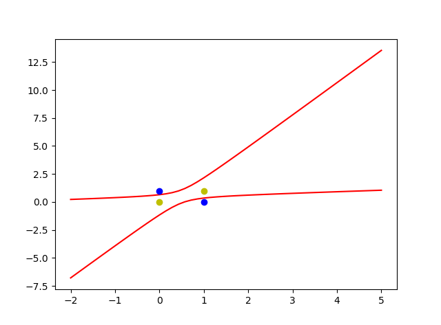
‘’‘’‘’

 浙公网安备 33010602011771号