

《python深度学习》笔记---5.4-2、卷积网络可视化-过滤器
《python深度学习》笔记---5.4-2、卷积网络可视化-过滤器
一、总结
一句话总结:
【每一层都学习一组过滤器】:卷积神经网络中每一层都学习一组过滤器,以便将其输入表示为过滤器的组合。
【过滤器变得越来越复杂,越来越精细】:这类似于傅里叶变换将信号分解为一 组余弦函数的过程。随着层数的加深,卷积神经网络中的过滤器变得越来越复杂,越来越精细。
【低层 对应简单的方向边缘和颜色】:模型第一层(block1_conv1)的过滤器对应简单的方向边缘和颜色(还有一些是彩色 边缘)。
【高层 类似于自然图像中的纹理:羽毛、眼睛、树叶等】:block2_conv1 层的过滤器对应边缘和颜色组合而成的简单纹理。更高层的过滤器类似于自然图像中的纹理:羽毛、眼睛、树叶等。
二、5.4-2、卷积网络可视化-过滤器
博客对应课程的视频位置:
Visualizing convnet filters
Another easy thing to do to inspect the filters learned by convnets is to display the visual pattern that each filter is meant to respond to. This can be done with gradient ascent in input space: applying gradient descent to the value of the input image of a convnet so as to maximize the response of a specific filter, starting from a blank input image. The resulting input image would be one that the chosen filter is maximally responsive to.
The process is simple: we will build a loss function that maximizes the value of a given filter in a given convolution layer, then we will use stochastic gradient descent to adjust the values of the input image so as to maximize this activation value. For instance, here's a loss for the activation of filter 0 in the layer "block3_conv1" of the VGG16 network, pre-trained on ImageNet:
from keras.applications import VGG16
from keras import backend as K

model = VGG16(weights='imagenet',
              include_top=False)

layer_name = 'block3_conv1'
filter_index = 0

layer_output = model.get_layer(layer_name).output
loss = K.mean(layer_output[:, :, :, filter_index])
To implement gradient descent, we will need the gradient of this loss with respect to the model's input. To do this, we will use the gradients function packaged with the backend module of Keras:
# The call to `gradients` returns a list of tensors (of size 1 in this case)
# hence we only keep the first element -- which is a tensor.
grads = K.gradients(loss, model.input)[0]
A non-obvious trick to use for the gradient descent process to go smoothly is to normalize the gradient tensor, by dividing it by its L2 norm (the square root of the average of the square of the values in the tensor). This ensures that the magnitude of the updates done to the input image is always within a same range.
# We add 1e-5 before dividing so as to avoid accidentally dividing by 0.
grads /= (K.sqrt(K.mean(K.square(grads))) + 1e-5)
Now we need a way to compute the value of the loss tensor and the gradient tensor, given an input image. We can define a Keras backend function to do this: iterate is a function that takes a Numpy tensor (as a list of tensors of size 1) and returns a list of two Numpy tensors: the loss value and the gradient value.
iterate = K.function([model.input], [loss, grads])

# Let's test it:
import numpy as np
loss_value, grads_value = iterate([np.zeros((1, 150, 150, 3))])
At this point we can define a Python loop to do stochastic gradient descent:
# We start from a gray image with some noise
input_img_data = np.random.random((1, 150, 150, 3)) * 20 + 128.

# Run gradient ascent for 40 steps
step = 1.  # this is the magnitude of each gradient update
for i in range(40):
    # Compute the loss value and gradient value
    loss_value, grads_value = iterate([input_img_data])
    # Here we adjust the input image in the direction that maximizes the loss
    input_img_data += grads_value * step
The resulting image tensor will be a floating point tensor of shape (1, 150, 150, 3), with values that may not be integer within [0, 255]. Hence we would need to post-process this tensor to turn it into a displayable image. We do it with the following straightforward utility function:
def deprocess_image(x):
    # normalize tensor: center on 0., ensure std is 0.1
    x -= x.mean()
    x /= (x.std() + 1e-5)
    x *= 0.1

    # clip to [0, 1]
    x += 0.5
    x = np.clip(x, 0, 1)

    # convert to RGB array
    x *= 255
    x = np.clip(x, 0, 255).astype('uint8')
    return x
Now we have all the pieces, let's put them together into a Python function that takes as input a layer name and a filter index, and that returns a valid image tensor representing the pattern that maximizes the activation the specified filter:
def generate_pattern(layer_name, filter_index, size=150):
    # Build a loss function that maximizes the activation
    # of the nth filter of the layer considered.
    layer_output = model.get_layer(layer_name).output
    loss = K.mean(layer_output[:, :, :, filter_index])

    # Compute the gradient of the input picture wrt this loss
    grads = K.gradients(loss, model.input)[0]

    # Normalization trick: we normalize the gradient
    grads /= (K.sqrt(K.mean(K.square(grads))) + 1e-5)

    # This function returns the loss and grads given the input picture
    iterate = K.function([model.input], [loss, grads])

    # We start from a gray image with some noise
    input_img_data = np.random.random((1, size, size, 3)) * 20 + 128.

    # Run gradient ascent for 40 steps
    step = 1.
    for i in range(40):
        loss_value, grads_value = iterate([input_img_data])
        input_img_data += grads_value * step

    img = input_img_data[0]
    return deprocess_image(img)
Let's try this:
plt.imshow(generate_pattern('block3_conv1', 0))
plt.show()

It seems that filter 0 in layer block3_conv1 is responsive to a polka dot pattern.
Now the fun part: we can start visualising every single filter in every layer. For simplicity, we will only look at the first 64 filters in each layer, and will only look at the first layer of each convolution block (block1_conv1, block2_conv1, block3_conv1, block4_conv1, block5_conv1). We will arrange the outputs on a 8x8 grid of 64x64 filter patterns, with some black margins between each filter pattern.
for layer_name in ['block1_conv1', 'block2_conv1', 'block3_conv1', 'block4_conv1']:
    size = 64
    margin = 5

    # This a empty (black) image where we will store our results.
    results = np.zeros((8 * size + 7 * margin, 8 * size + 7 * margin, 3))

    for i in range(8):  # iterate over the rows of our results grid
        for j in range(8):  # iterate over the columns of our results grid
            # Generate the pattern for filter `i + (j * 8)` in `layer_name`
            filter_img = generate_pattern(layer_name, i + (j * 8), size=size)

            # Put the result in the square `(i, j)` of the results grid
            horizontal_start = i * size + i * margin
            horizontal_end = horizontal_start + size
            vertical_start = j * size + j * margin
            vertical_end = vertical_start + size
            results[horizontal_start: horizontal_end, vertical_start: vertical_end, :] = filter_img

    # Display the results grid
    plt.figure(figsize=(20, 20))
    plt.imshow(results)
    plt.show()
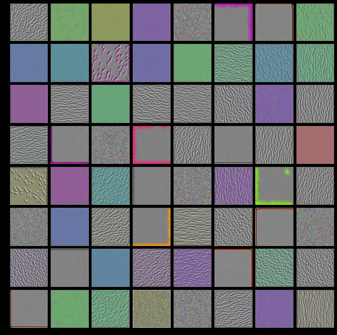
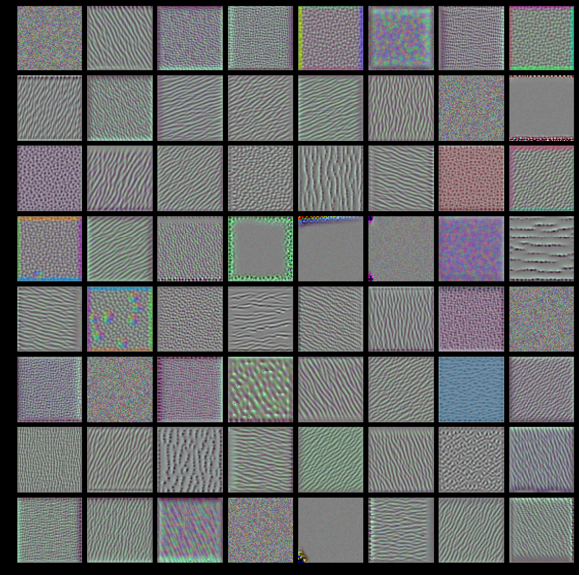


These filter visualizations tell us a lot about how convnet layers see the world: each layer in a convnet simply learns a collection of filters such that their inputs can be expressed as a combination of the filters. This is similar to how the Fourier transform decomposes signals onto a bank of cosine functions. The filters in these convnet filter banks get increasingly complex and refined as we go higher-up in the model:
- The filters from the first layer in the model (
block1_conv1) encode simple directional edges and colors (or colored edges in some cases). - The filters from
block2_conv1encode simple textures made from combinations of edges and colors. - The filters in higher-up layers start resembling textures found in natural images: feathers, eyes, leaves, etc.

 浙公网安备 33010602011771号