ML03 LinearRegression_byMyself

ML实战：手动实现梯度下降法线性回归

• 本次实验使用的数据集是自己编写

/*prices.txt*/
1000,168
792,184
1260,197
1262,220
1240,228
1170,248
1230,305
1255,256
1194,240
1450,230
1481,202
1475,220
1482,232
1484,460
1512,320
1680,340
1620,240
1720,368
1800,280
4400,710
4212,552
3920,580
3212,585
3151,590
3100,560
2700,285
2612,292
2705,482
2570,462
2442,352
2387,440
2292,462
2308,325
2252,298
2202,352
2157,403
2140,308
4000,795
4200,765
3900,705
3544,420
2980,402
4355,762
3150,392

代码实现

import numpy as np
import sys
import matplotlib.pyplot as plt
from sklearn.model_selection import train_test_split

np.set_printoptions(suppress=True)


def h(x,theta):
    #假设函数，计算h(x)
    return np.matmul(x,theta)

def single_iter(x,y,theta,alpha):
    #单次迭代，计算每个theta的值
    theta_size=len(theta)
    size=len(x)
    res=h(x,theta)
    res=res-y
    for i in range(theta_size):
        temp=theta[i][0]
        temp=temp-alpha/size*(np.matmul(x[:,i],res))
        theta[i]=temp
    print(theta)

def gradient_decend(x,y,theta,alpha=0.3,iter_count=500):
    #迭代函数,默认学习率为0.3，迭代次数为500
    for i in range(iter_count):
        single_iter(x,y,theta,alpha)

def predict(x):
    #预测函数
    return x*theta[1][0]+theta[0][0]

def showres(x,y):
    #结果显示
    minx=np.min(x)
    maxx=np.max(x)
    y_1=y.T[0]
    x_1=x.T[1]
    X=np.arange(minx,maxx).reshape([-1,1])
    plt.figure(figsize=(20,8),dpi=80)
    plt.scatter(x_1,y_1,color='blue')
    plt.plot(X,predict(X),color='red')
    #plt.savefig('E:/Python/ml/pic/Linear_of_GradientDecend_myself.png')

#初始化数据以及theta参数
fr=open('E:\Python\ml\课程数据\回归\prices.txt','r')
lines=fr.readlines()
x=[]
y=[]
for line in lines:
    item=line.split(',')
    x.append(1)
    x.append(int(item[0]))
    y.append(int(item[1]))
x=np.array(x,dtype=float).reshape((-1,2))
y=np.array(y,dtype=float).reshape((-1,1))

theta=np.random.rand(len(x[0]),1)
theta[0]=1
x_train,x_test,y_train,y_test=train_test_split(x,y,test_size=0.3,random_state=np.random.randint(0,30))



gradient_decend(x_train,y_train,theta,0.0000001)
showres(x_test,y_test)

sys.exit(0)

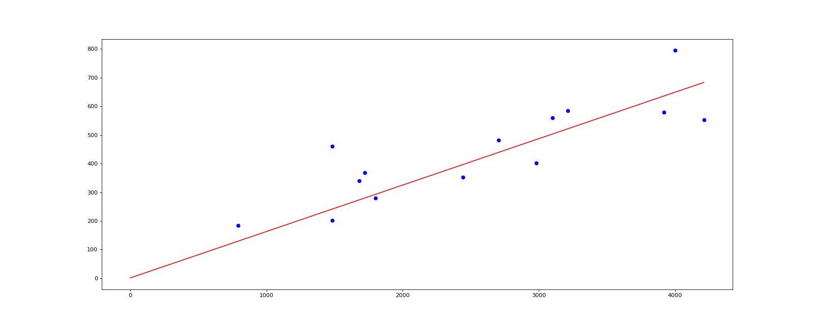
结果

总结

• 最深有感触的就是学习率的问题
• 为什么我默认α=0.3，但是却在实现中把α设置为0.0000001？
  • 因为本次实验的输入数据集没有实现标准化，因此x过于离散，使用α过大（哪怕是0.0001）也会导致最终θ数组发散
• 后续会把以上方法封装成类，应用到波士顿房价数据集上。