

【ANSYS学习笔记】Case03_Basic Electrostatic Analysis_基本静电分析
• Introduction on the Electrostatic Solver
– This workshop introduces the Electro Static solver based on some simple examples. This solver is meant to solve the static electric field without current flowing in conductors (conductors are in electrostatic equilibrium). The conductors are considered perfect such that there is no electric field inside conductors.
Electrostatic求解器用于解决静电场而无需电流在导体中流动的问题,导体处于静电平衡状态。在该解算器重,导体认为是理想的,因此认为导体内部没有电场。
Example1: Cylindrical Capacitor in RZ
• In this example, we will determine the electric field distribution of coaxial cable based on the potential (or the charges) that are applied on each conductor. Coaxial cable will be solved with RZ representation
分析同轴电缆的电场分布,同轴电缆通过RZ坐标轴进行建模。
Step01: 建立工程文档,配置工程
• Create Design
– Select the menu item Project Insert Maxwell 2D Design,
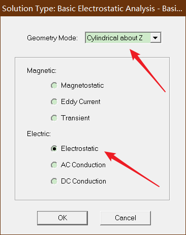
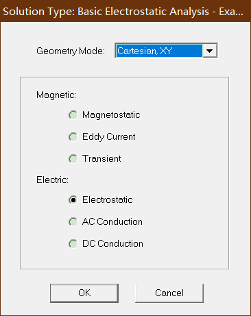
• Set Solution Type
– Select the menu item Maxwell 2D Solution Type
– Solution Type Window:
1. Geometry Mode: Cylindrical about Z
2. Choose Electric > Electrostatic
3. Click the OK button

Step02:Create Model 创建模型
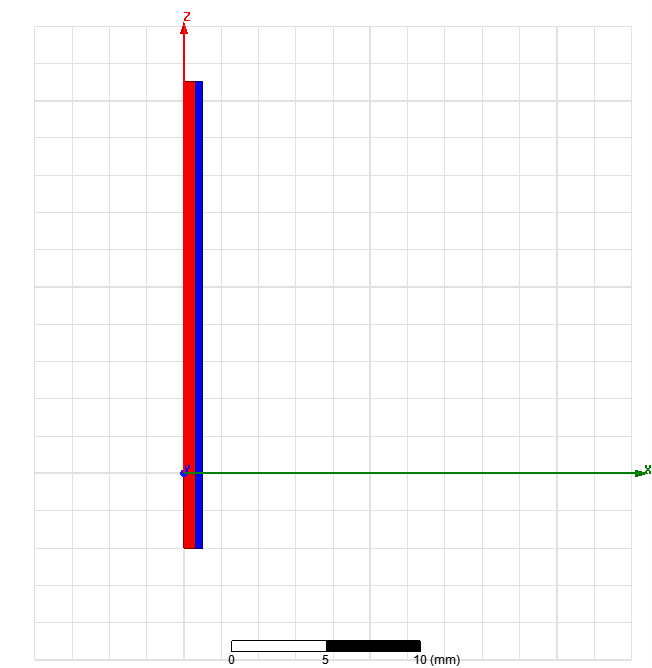
• Create object Inner
– Select the menu item Draw Rectangle
1. Using the coordinate entry fields, enter the position of rectangle
– X: 0, Y: 0, Z: -4, Press the Enter key
2. Using the coordinate entry fields, enter the opposite corner
– dX: 0.6, dY: 0, dZ: 25, Press the Enter key
– Change the name of resulting sheet to Inner and color to Light Red
– Change the material of the sheet to Copper

• Create Air Gap
– Select the menu item Draw Rectangle
1. Using the coordinate entry fields, enter the position of rectangle
– X: 0.6, Y: 0, Z: -4, Press the Enter key
2. Using the coordinate entry fields, enter the opposite corner
– dX: 0.4, dY: 0, dZ: 25, Press the Enter key
– Change the name of resulting sheet to Air and color to Light Blue
– Change the material of the sheet to air
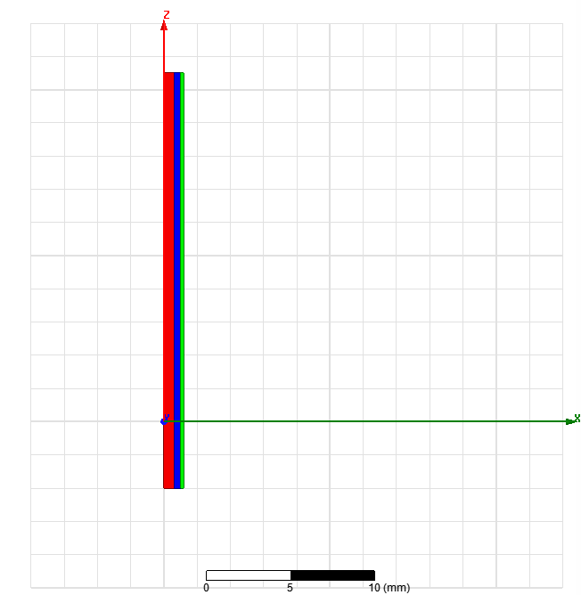
• Create object outer
– Select the menu item Draw Rectangle
1. Using the coordinate entry fields, enter the position of rectangle
– X: 1, Y: 0, Z: -4, Press the Enter key
2. Using the coordinate entry fields, enter the opposite corner
– dX: 0.2, dY: 0, dZ: 25, Press the Enter key
– Change the name of resulting sheet to Outer and color to Light Green
– Change the material of the sheet to Copper
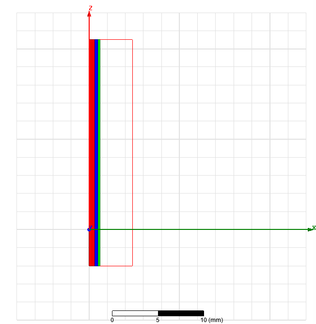
• Create Simulation Region
– Select the menu item Draw Region
– In Region window,
1. Pad individual directions: Checked
2. Padding Type: Percentage Offset
– +R = 300
– Specify rest to 0
3. Press OK
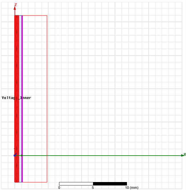
Step03:Assign Excitations:分配激励
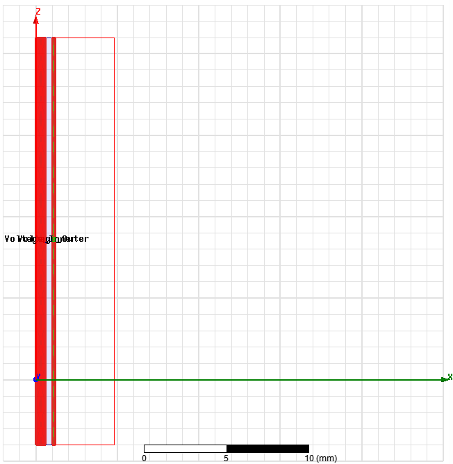
• Assign Excitation to object Inner
– Select the sheet Inner from the history tree
– Select the menu item Maxwell 2D Excitations Assign Voltage
– In Voltage Excitation window,
• Name: Voltage_Inner
• Value: -1kV
• Press OK
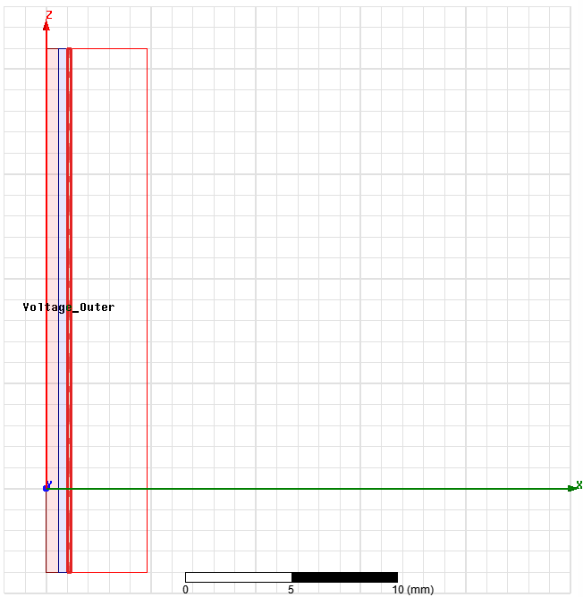
• Assign Excitation to object Outer
– Select the sheet Outer from the history tree
– Select the menu item Maxwell 2D Excitations Assign Voltage
– In Voltage Excitation window,
• Name: Voltage_Outer
• Value: 1kV
• Press OK
Step04:Assign Executive Parameters:分配执行参数
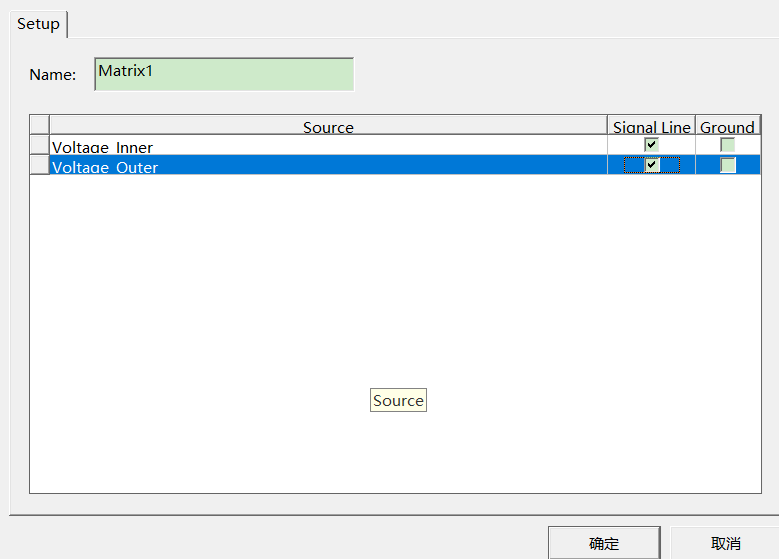
• Assign Capacitance Computation
– Select the menu item Maxwell2D Parameters Assign Matrix
– In Matrix window
1. Voltage_Inner and Voltage_Outer
– Signal Line: Checked
2. Press OK
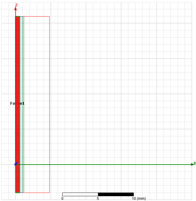
• Assign Force Computation
– Select the sheet Inner from history tree
– Select the menu item Maxwell 2D Parameters Assign Force
– In Force Setup window, press OK
Step05:Analyze
• Create an analysis setup:
– Select the menu item Maxwell 2D Analysis Setup Add Solution Setup
– Solution Setup Window:
1. General Tab
– Percentage Error: 0.5
2. Convergence Tab
– Refinement Per Pass: 50%
3. Click the OK button
• Start the solution process:
– Select the menu item Maxwell 2DAnalyze All
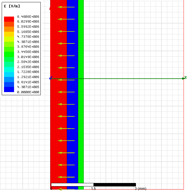
Step06:Plot Electric Field Vectors
• Plot Electric Field Vectors
– Select the Plane Global:XZ from history tree
– Select the menu item Maxwell 2D Fields Fields E E_Vector
– In Create Field Plot window,
• Press Done
– To adjust spacing and size of arrows, double click on the legend and then go to
Marker/Arrow and Plots tabs
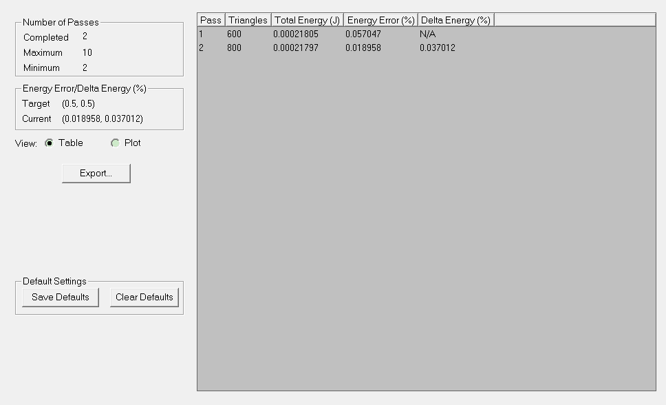
Step07: View Results
• View Results
– Select the menu item Maxwell 2D Results Solution Data
– In Solutions window
• Select Force tab
– Note: The force is zero since the model is magnetically balanced.
• Select Matrix tab
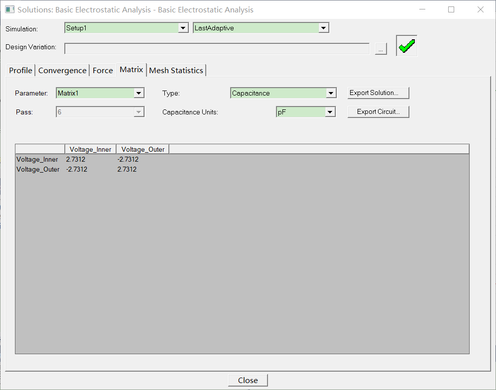
– The analytical value of the capacitance per meter for an infinite long coaxial wire
is given by the following formula:
C = 2πε0 / ln(b/a) (a and b being the inside and outside diameters)
– The analytical value would is therefore 1.089e-10 F/m (a =0.6mm, b=1mm)
– In our project, length of the conductor is 25 mm, therefore the total capacitance is. 2.723pF. We obtain a good agreement with the obtained result 2.7312 pF.
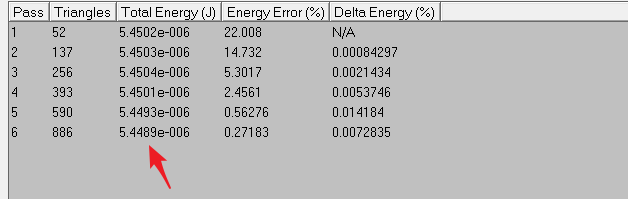
in the Convergence tab, you have access to the total energy of the system. We find 5.4489e-6 J. It is exactly 2000 times the capacitance (2000V being the difference of potential).
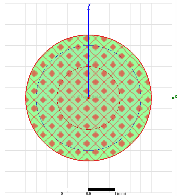
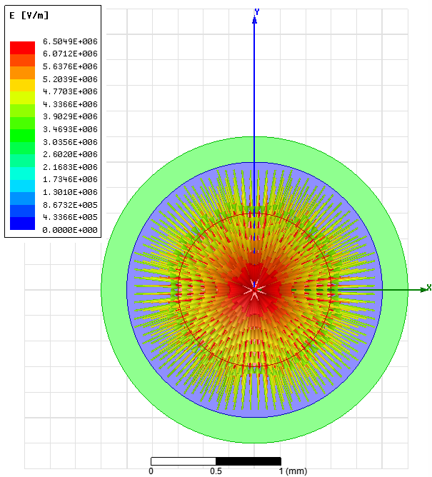
Example2: Cylindrical Capacitor in XY
• The same problem will now solved using an XY representation
Step01:建立工程文件,并进行基本配置
• Create Design
– Select the menu item Project Insert Maxwell 2D Design, or click on the
icon
• Set Solution Type
– Select the menu item Maxwell 2D Solution Type
– Solution Type Window:
1. Geometry Mode: Cartesian, XY
2. Choose Electric > Electrostatic
3. Click the OK button
Step02:Create Model 建模
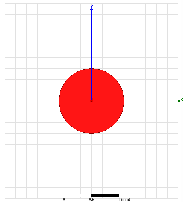
• Create Object Inner
– Select the menu item Draw Circle
1. Using the coordinate entry fields, enter the center of circle
– X: 0, Y: 0, Z: 0, Press the Enter key
2. Using the coordinate entry fields, enter the radius
– dX: 0.6, dY: 0, dZ: 0, Press the Enter key
– Change the name of resulting sheet to Inner and color to Light Red
– Change the material of the sheet to Copper
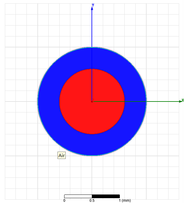
• Create Air Gap
– Select the menu item Draw Circle
1. Using the coordinate entry fields, enter the center of circle
– X: 0, Y: 0, Z: 0, Press the Enter key
2. Using the coordinate entry fields, enter the radius
– dX: 1.0, dY: 0, dZ: 0, Press the Enter key
– Change the name of resulting sheet to Air and color to Light Blue
– Change the material of the sheet to air
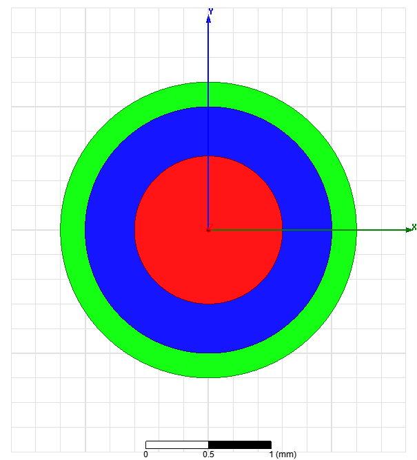
• Create Object Outer
– Select the menu item Draw Circle
1. Using the coordinate entry fields, enter the center of circle
– X: 0, Y: 0, Z: 0, Press the Enter key
2. Using the coordinate entry fields, enter the radius
– dX: 1.2, dY: 0, dZ: 0, Press the Enter key
– Change the name of resulting sheet to Outer and color to Light Green
– Change the material of the sheet to Copper
Step03:Assign Excitations 添加激励
• Assign Excitation to object Inner
– Select the sheet Inner from the history tree
– Select the menu item Maxwell 2D Excitations Assign Voltage
– In Voltage Excitation window,
• Name: Voltage_Inner
• Value: -1kV
• Press OK
• Assign Excitation to object Outer
– Select the sheet Outer from the history tree
– Select the menu item Maxwell 2D Excitations Assign Voltage
– In Voltage Excitation window,
• Name: Voltage_Outer
• Value: 1kV
• Press OK
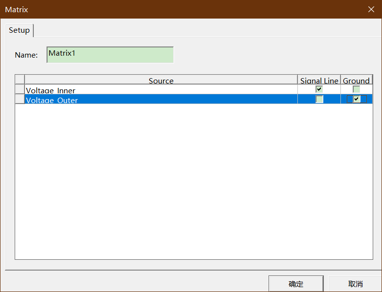
Step04:Assign Executive Parameters
• Assign Capacitance Computation
– Select the menu item Maxwell2D Parameters Assign Matrix
– In Matrix window
1. Voltage_Inner
– Signal Line: Checked
2. Voltage_Outer
– Ground: Checked
3. Press OK
– We ground Voltage_Outer. We will obtain just a 1 by 1 matrix.
Step05:Analyze
• Create an analysis setup:
– Select the menu item Maxwell 2D Analysis Setup Add Solution Setup
– Solution Setup Window:
1. General Tab
– Percentage Error: 0.5
2. Convergence Tab
– Refinement Per Pass: 50%
3. Click the OK button
• Start the solution process:
– Select the menu item Maxwell 2DAnalyze All
Step06:View Results
• View Capacitance
– Select the menu item Maxwell 2D Results Solution Data
– In Solutions window
• Select Matrix tab
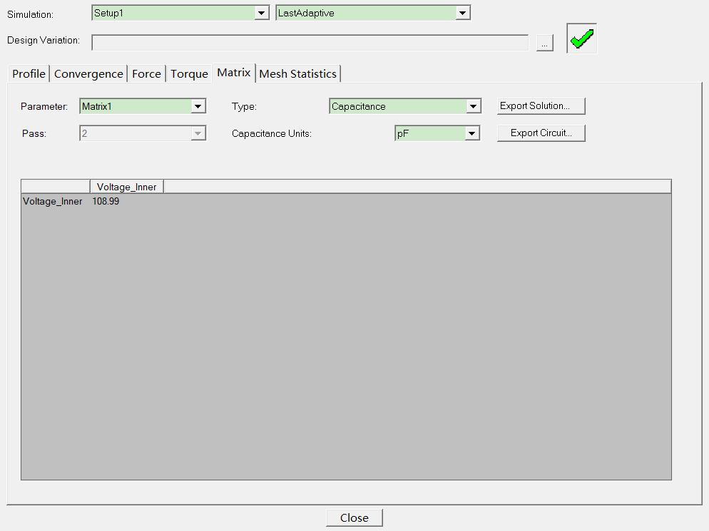
– The analytical value of the capacitance per meter for an infinite long coaxial wire
is given by the following formula:
C = 2πε0 / ln(b/a) (a and b being the inside and outside diameters)
– The analytical value would be therefore 1.089e-10 F/m (a =0.6mm, b=1mm)
– This matches the obtained value.
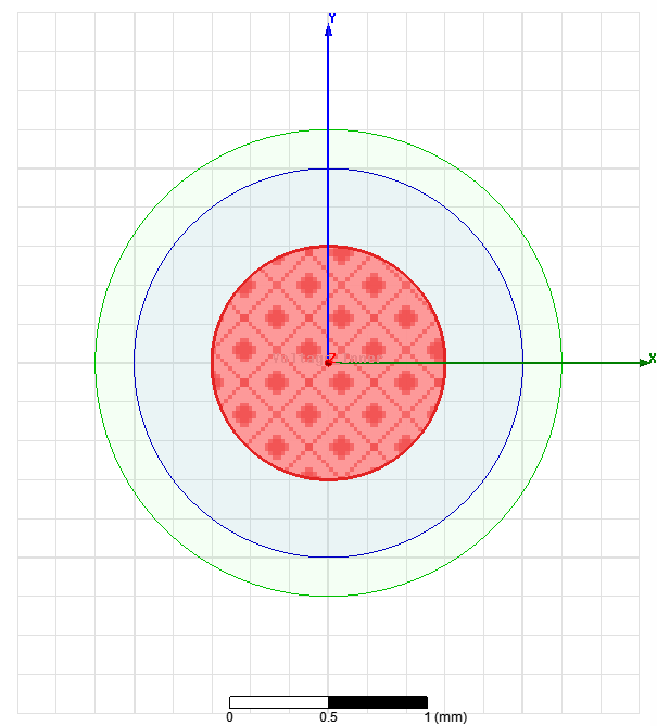
Step07:Plot Electric Field Vectors
• Plot Electric Field Vectors
– Select the Plane Global:XZ from history tree
– Select the menu item Maxwell 2D Fields Fields E E_Vector
– In Create Field Plot window,
• Press Done
– To adjust spacing and size of arrows, double click on the legend and then go to
Marker/Arrow and Plots tabs
Example3: Capacitance of a Planar Capacitor
• In this example we illustrate how to simulate a simple planar capacitor made of two parallel plates
Step01:建立工程,并进行设置
• Create Design
– Select the menu item Project Insert Maxwell 2D Design, or click on the
icon
• Set Solution Type
– Select the menu item Maxwell 2D Solution Type
– Solution Type Window:
1. Geometry Mode: Cartesian, XY
2. Choose Electric > Electrostatic
3. Click the OK button
Step02:Create Model 建模
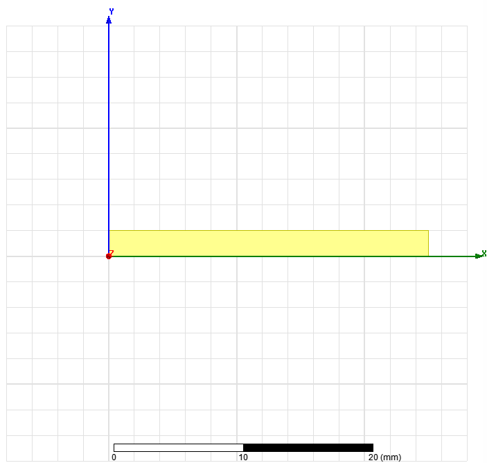
• Create Object DownPlate
– Select the menu item Draw Rectangle
1. Using the coordinate entry fields, enter the position of rectangle
– X: 0, Y: 0, Z: 0, Press the Enter key
2. Using the coordinate entry fields, enter the opposite corner
– dX: 25, dY: 2, dZ: 0, Press the Enter key
– Change the name of resulting sheet to DownPlate and color to Yellow
– Change the material of the sheet to Copper
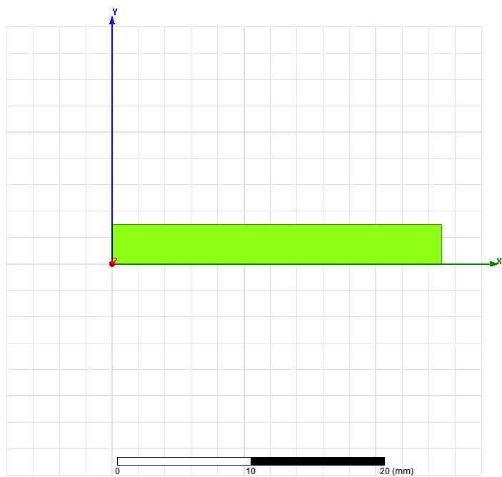
• Create Object Region
– Select the menu item Draw Rectangle
1. Using the coordinate entry fields, enter the position of rectangle
– X: 0, Y: 0, Z: 0, Press the Enter key
2. Using the coordinate entry fields, enter the opposite corner
– dX: 25, dY: 3, dZ: 0, Press the Enter key
– Change the name of resulting sheet to Region and color to Green
– Change the material of the sheet to air
Step03:Assign Excitations 分配激励
• Assign Excitation to object DownPlate
– Select the sheet DownPlate from the history tree
– Select the menu item Maxwell 2D Excitations Assign Voltage
– In Voltage Excitation window,
• Value: 0 V
• Press OK

• Assign Excitation to Region
– Select the menu item Edit Select Edges
– Select the top edge of the Region as shown in below image
– Select the menu item Maxwell 2D Excitations Assign Voltage
– In Voltage Excitation window,
• Value: 1 V
• Press OK

Step04:Assign Executive Parameters
• Assign Capacitance Computation
– Select the menu item Maxwell2D Parameters Assign Matrix
– In Matrix window
1. Voltage1
– Signal Line: Checked
2. Voltage2
– Ground: Checked
3. Press OK
Step05:Analyze
• Create an analysis setup:
– Select the menu item Maxwell 2D Analysis Setup Add Solution Setup
– Solution Setup Window:
1. General Tab
– Percentage Error: 1
2. Convergence Tab
– Refinement Per Pass: 50%
3. Click the OK button
• Start the solution process:
– Select the menu item Maxwell 2DAnalyze All
Step06:View Results
• View Capacitance
– Select the menu item Maxwell 2D Results Solution Data
– In Solutions window
• Select Matrix tab
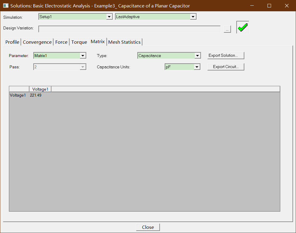
– The analytical value of the capacitance for two parallel plates is given by:
C = A/ d *ε0 (A is the area of the plate and d is the thickness of the di electrics)
– If we consider the plate to be 25mm by 25 mm, using the above formula, we obtain 5.53 pF (the dielectric is 1mm thick).
– We obtain 221.49pF. This value should be considered as the capacitance of the two parallel plates with a 1 meter depth. If we rescale this value by multiplying
by 0.025m (25 mm) we find 5.53pF as well.
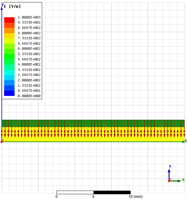
Step07:Plot Electric Field Vectors
• Plot Electric Field Vectors
– Select the Plane Global:XZ from history tree
– Select the menu item Maxwell 2D Fields Fields E E_Vector
– In Create Field Plot window,
• Press Done
– To adjust spacing and size of arrows, double click on the legend and then go to
Marker/Arrow and Plots tabs

 浙公网安备 33010602011771号