游乐园日志_使用媒体营销活动成本数据集的表格回归
关于数据集
Food Mart(CFM)是美国的一家连锁便利店。这家私营公司的总部位于俄亥俄州的门托市,目前,在美国大约有325家商店。便利食品超市采用特许经营制度运作。
截至1988年,Food Mart是美国第三大的连锁便利店。
同年,纳斯达克交易所因该公司未能达到财务报告的要求而放弃了便利食品市场。
在20世纪80年代,卡登和切瑞公司用欧内斯特的形象为便利食品市场做广告。
你的任务是设计一个机器学习模型,帮助我们根据所提供的特征来预测食品市场的媒体活动成本。
数据集描述
store_sales(in millions) - 商店销售额(单位:百万美元)
unit_sales(in millions) - 商店的单位销售量(单位:百万) 数量
Total_children - 家庭中的儿童总数
avg_cars_at home(约) - avg_cars_at home(约)
Num_children_at_home - 根据客户填写的信息,在家的孩子数量
Gross_weight - 物品的总重量
Recyclable_package - 食品项目是可回收包装的。
Low_fat - 低脂肪食品项目是低脂肪的。
Units_per_case - 每家商店货架上可提供的单位/箱数。
Store_sqft - 可用的商店面积,以平方尺计。
Coffee_bar - 店内有咖啡吧。
Video_store - 可提供视频商店/游戏商店
Salad_bar - 店内有沙拉吧。
预制食品 - 店内有预制食品
花店 - 店内有鲜花货架
成本 - 吸引顾客的成本,单位为美元
编辑
数据集描述
本次竞赛的数据集(训练和测试)是根据在媒体营销活动成本预测数据集上训练的深度学习模型生成的。特征分布与原始分布接近,但不完全相同。随意使用原始数据集作为本次竞赛的一部分,既可以探索差异,也可以了解在训练中合并原始数据集是否可以提高模型性能。
文件
- 训练.csv - 训练数据集; 是目标
cost - 测试.csv - 测试数据集;您的目标是预测
cost - sample_submission.csv - 正确格式的示例提交文件
均方根对数误差 (RMLSE)
提交的内容根据均方根对数误差 (RMSLE) 进行评分(sklearn with )。mean_squared_log_error``squared=False
成绩: 0.29897 当前排名461
提交文件
对于测试集中的每个值,必须预测目标 的值。该文件应包含标头并具有以下格式:id-``cost
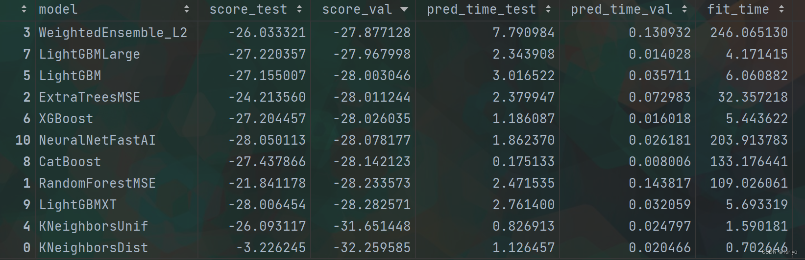
模型性能比较:
编辑
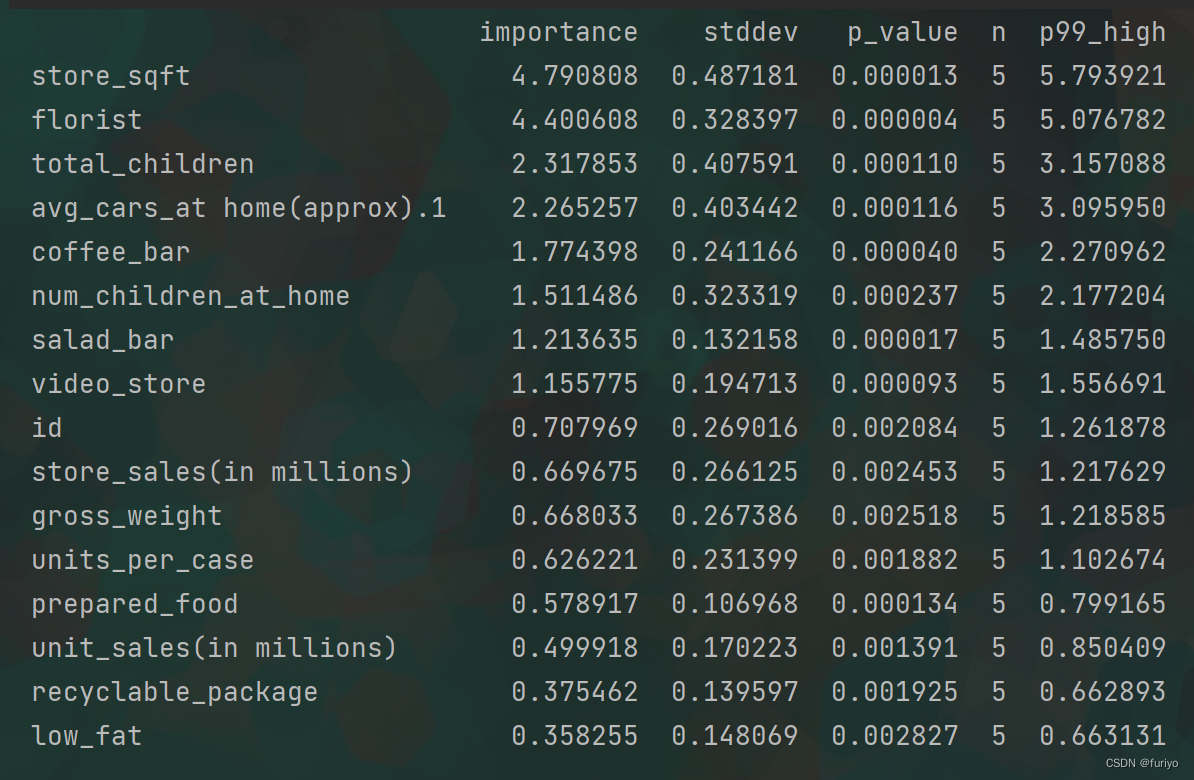
特征重要程度:
编辑
stddev:这是标准差的简称,是对一组数据中的变化量或分散度的测量。它经常被用来描述一个分布的范围。
p_value: 这是一种统计学措施,有助于确定一个特定结果或发现的重要性。它表示在假设无效假设(即没有影响或关系)为真时,获得与观察到的结果一样极端或更极端的概率。
p99_high(low): 这可能是指分布中的第99个百分位数,它代表了99%的数据低于这个值。高和低的修饰语表明这是指分布的上端或下端。
notebook:
Abstract:
This notebook present a beginner approach to episode 11 of season 3 playground series which is about Tabular Regression with a Media Campaign Cost Dataset.
Simple explanatory data analysis was performed to evaluate features.
Original dataset was added to the synthetic set
Feature selection was conducted based on @tolgayan notebook
- Turns out that removing low_fat impoves the LB score.
Feature engineering was performed to introduce some relevent features.
- Multiple features were added but it seemed that [ 'children_per_adult','independent_children', 'child_to_car_ratio' , 'any_amenities' ] had a better effect on the score.
Some of the simple regression models and tree ensemble based models with default hyperparameters were used for modeling to choose a baseline model based on RMSLE metrics.
- Despite the long computational cost neural network didn't provide a good prediction.
- Random Forrest regression showed the best prediction.
- Mixing the results of diffrent models seemed effective in increasing the score. For instance, considering the results of Random forest with 0.7 weight and adding the results of Xgboost with 0.3 weight slightly improved the prediction.
Hyperparameters of the models were tuned to increase the accuracy.
- Some Hyperparameters tunnin were done to increase the LB wih Xgboost model.
- Kfold cross validation method showed slight improvement to LB score.
结果发现,去除low_fat会影响LB的得分。
进行了特征工程以引入一些相关的特征。
添加了多个特征,但似乎['children_per_adult', 'independent_children', 'child_to_car_ratio', 'any_amenities']对得分有更好的影响。
一些简单的回归模型和基于默认超参数的树状集合模型被用于建模,以选择一个基于RMSLE指标的基线模型。
尽管计算成本较高,但神经网络并没有提供良好的预测结果。
随机福斯特回归显示了最好的预测结果。
混合不同模型的结果似乎可以有效地提高分数。例如,考虑到权重为0.7的随机森林的结果,再加上权重为0.3的Xgboost的结果,预测效果略有提高。
对模型的超参数进行了调整以提高准确性。
一些超参数的调整是为了提高Xgboost模型的准确率。
Kfold交叉验证方法显示了对LB分数的轻微改善。
About Dataset:
- Original dataset is about Food Mart (CFM), a chain of convenience stores in the United States.
- Task is to devise a Machine Learning Model that helps us predict the cost of media campaigns in the food marts on the basis of the features provided.
- The dataset for this competition (both train and test) was generated from a deep learning model trained on the Media Campaign Cost Prediction dataset.
- Incorporating the original dataset in training might improve model performance.
- Import libraries
This section imports the main libraries which were used in this notebook.
In [1]:
import numpy as np
import pandas as pd
import matplotlib.pyplot as plt
import seaborn as sns

# Feature scaling if necessary
from sklearn.preprocessing import StandardScaler,MinMaxScaler

# To evaluate the model
from sklearn.metrics import make_scorer,mean_squared_log_error

# Linear regression
from sklearn.linear_model import LinearRegression

# Ridge regression
from sklearn.linear_model import Ridge

# Lasso regression
from sklearn.linear_model import Lasso

# Random Forrest Regressor
from sklearn.ensemble import RandomForestRegressor

# xgboost model and feature importance
from xgboost import XGBRegressor,plot_importance

# lightgbm model
from lightgbm import LGBMRegressor

# catboost Regressor model
from catboost import CatBoostRegressor

# Extra Trees Regressor model
from sklearn.ensemble import ExtraTreesRegressor

# Tuning hyperparameters
from sklearn.model_selection import GridSearchCV

RANDOM_STATE = 17
- Loading data
In [2]:
# Playground dataset train & test
P_train_df = pd.read_csv('/kaggle/input/playground-series-s3e11/train.csv')
P_test_df = pd.read_csv('/kaggle/input/playground-series-s3e11/test.csv')

# Original dataset train & test
O_test_df = pd.read_csv('/kaggle/input/media-campaign-cost-prediction/test_dataset.csv')
O_train_df = pd.read_csv('/kaggle/input/media-campaign-cost-prediction/train_dataset.csv')
In [3]:
P_train_df.head(2)
Out[3]:
| id | store_sales(in millions) | unit_sales(in millions) | total_children | num_children_at_home | avg_cars_at home(approx).1 | gross_weight | recyclable_package | low_fat | units_per_case | store_sqft | coffee_bar | video_store | salad_bar | prepared_food | florist | cost | |
|---|---|---|---|---|---|---|---|---|---|---|---|---|---|---|---|---|---|
| 0 | 0 | 8.61 | 3.0 | 2.0 | 2.0 | 2.0 | 10.30 | 1.0 | 0.0 | 32.0 | 36509.0 | 0.0 | 0.0 | 0.0 | 0.0 | 0.0 | 62.09 |
| 1 | 1 | 5.00 | 2.0 | 4.0 | 0.0 | 3.0 | 6.66 | 1.0 | 0.0 | 1.0 | 28206.0 | 1.0 | 0.0 | 0.0 | 0.0 | 0.0 | 121.80 |
In [4]:
O_train_df.head(2)
Out[4]:
| store_sales(in millions) | unit_sales(in millions) | total_children | num_children_at_home | avg_cars_at home(approx).1 | gross_weight | recyclable_package | low_fat | units_per_case | store_sqft | coffee_bar | video_store | salad_bar | prepared_food | florist | cost | |
|---|---|---|---|---|---|---|---|---|---|---|---|---|---|---|---|---|
| 0 | 2.68 | 2.0 | 1.0 | 0.0 | 2.0 | 6.3 | 1.0 | 0.0 | 22.0 | 30584.0 | 1.0 | 1.0 | 1.0 | 1.0 | 1.0 | 79.59 |
| 1 | 5.73 | 3.0 | 5.0 | 5.0 | 3.0 | 18.7 | 1.0 | 0.0 | 30.0 | 20319.0 | 0.0 | 0.0 | 0.0 | 0.0 | 0.0 | 118.36 |
In [5]:
P_test_df.head(2)
Out[5]:
| id | store_sales(in millions) | unit_sales(in millions) | total_children | num_children_at_home | avg_cars_at home(approx).1 | gross_weight | recyclable_package | low_fat | units_per_case | store_sqft | coffee_bar | video_store | salad_bar | prepared_food | florist | |
|---|---|---|---|---|---|---|---|---|---|---|---|---|---|---|---|---|
| 0 | 360336 | 7.24 | 4.0 | 1.0 | 0.0 | 2.0 | 10.80 | 0.0 | 1.0 | 7.0 | 20319.0 | 0.0 | 0.0 | 0.0 | 0.0 | 0.0 |
| 1 | 360337 | 6.90 | 2.0 | 2.0 | 2.0 | 3.0 | 8.51 | 1.0 | 0.0 | 4.0 | 33858.0 | 1.0 | 0.0 | 1.0 | 1.0 | 1.0 |
In [6]:
print(f"Playground dataset has {P_train_df.shape[1]} features and {P_train_df.shape[0]} training examples.")
print(f"Original dataset has {O_train_df.shape[1]} features and {O_train_df.shape[0]} training examples.")
Playground dataset has 17 features and 360336 training examples.
Original dataset has 16 features and 51363 training examples.
In [7]:
P_train_df.info()
<class 'pandas.core.frame.DataFrame'>
RangeIndex: 360336 entries, 0 to 360335
Data columns (total 17 columns):
 #   Column                      Non-Null Count   Dtype
---  ------                      --------------   -----
 0   id                          360336 non-null  int64
 1   store_sales(in millions)    360336 non-null  float64
 2   unit_sales(in millions)     360336 non-null  float64
 3   total_children              360336 non-null  float64
 4   num_children_at_home        360336 non-null  float64
 5   avg_cars_at home(approx).1  360336 non-null  float64
 6   gross_weight                360336 non-null  float64
 7   recyclable_package          360336 non-null  float64
 8   low_fat                     360336 non-null  float64
 9   units_per_case              360336 non-null  float64
 10  store_sqft                  360336 non-null  float64
 11  coffee_bar                  360336 non-null  float64
 12  video_store                 360336 non-null  float64
 13  salad_bar                   360336 non-null  float64
 14  prepared_food               360336 non-null  float64
 15  florist                     360336 non-null  float64
 16  cost                        360336 non-null  float64
dtypes: float64(16), int64(1)
memory usage: 46.7 MB
- EDA
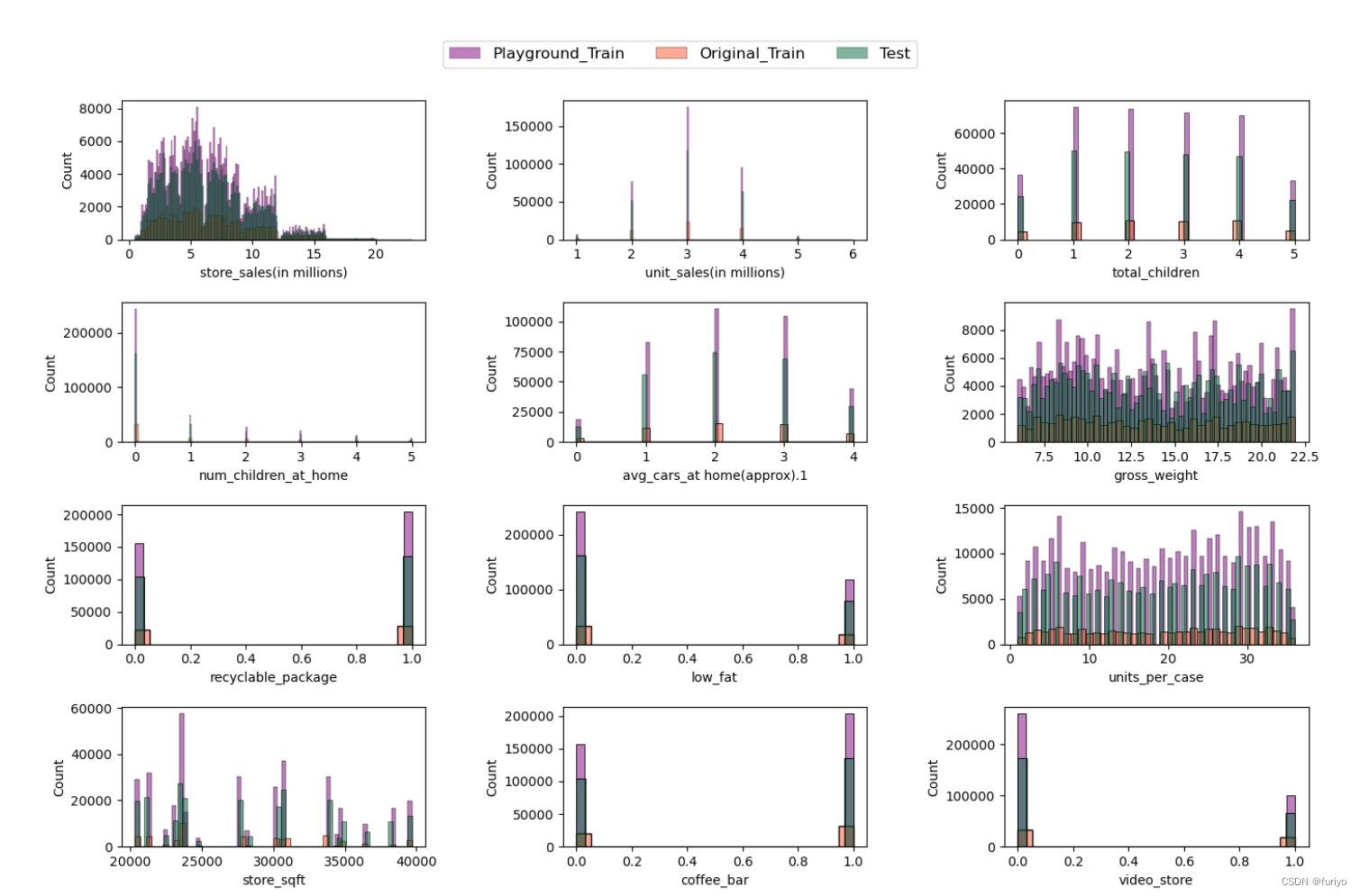
3.1 Feature distribution
First of all, It is recommended to evaluate the distribution of the train and test dataset. In this step histograms were created to show how each feature was distributed in a given dataset. After that Kernel density function was plotted to see the resemblance more vividly.
In [8]:
linkcode
# Create multiple plots with a given size
fig = plt.figure(figsize=(15,12))

features = P_train_df.columns[1:-1]

# Create a countplot to evaluate the distribution
for i, feature in enumerate(features):
    ax = plt.subplot(5, 3, i+1)
    sns.histplot(x=feature, data=P_train_df, label="Playground_Train", color='#800080', ax=ax, alpha=0.5)
    sns.histplot(x=feature, data=O_train_df, label="Original_Train", color='#FF5733', ax=ax, alpha=0.5)
    sns.histplot(x=feature, data=P_test_df, label="Test", color='#006b3c', ax=ax, alpha=0.5)
#     ax.set_xlabel(feature, fontsize=12)

# Create the legend
fig.legend(labels=['Playground_Train', 'Original_Train', 'Test'], loc='upper center', bbox_to_anchor=(0.5, 0.96), fontsize=12, ncol=3)

# Adjust the spacing between the subplots and the legend
fig.subplots_adjust(top=0.90, bottom=0.05, left=0.10, right=0.95, hspace=0.45, wspace=0.45)

plt.show()
编辑
# Create multiple plots
fig, axes = plt.subplots(nrows=5, ncols=3, figsize=(15,12))
fig.tight_layout(pad=2)

fig.subplots_adjust(top=0.85)  # adjust top margin to make space for legend

features = P_train_df.columns[1:-1]

# Create a countplot to evaluate the distribution
for i, feature in enumerate(features):
    row = i // 3
    col = i % 3
    ax = axes[row, col]
    sns.kdeplot(x=feature, data=P_train_df, label="Playground_Train", color='#800080', fill=True, ax=ax)
    sns.kdeplot(x=feature, data=O_train_df, label="Original_Train", color='#FF5733', fill=True, ax=ax)
    sns.kdeplot(x=feature, data=P_test_df, label="Test", color='#006b3c', fill=True, ax=ax)

fig.legend(labels=['Playground_Train', 'Original_Train', 'Test'], loc='upper center', bbox_to_anchor=(0.5, 0.96), fontsize=12, ncol=3)
Out[9]:
<matplotlib.legend.Legend at 0x7f0824243c50>
编辑
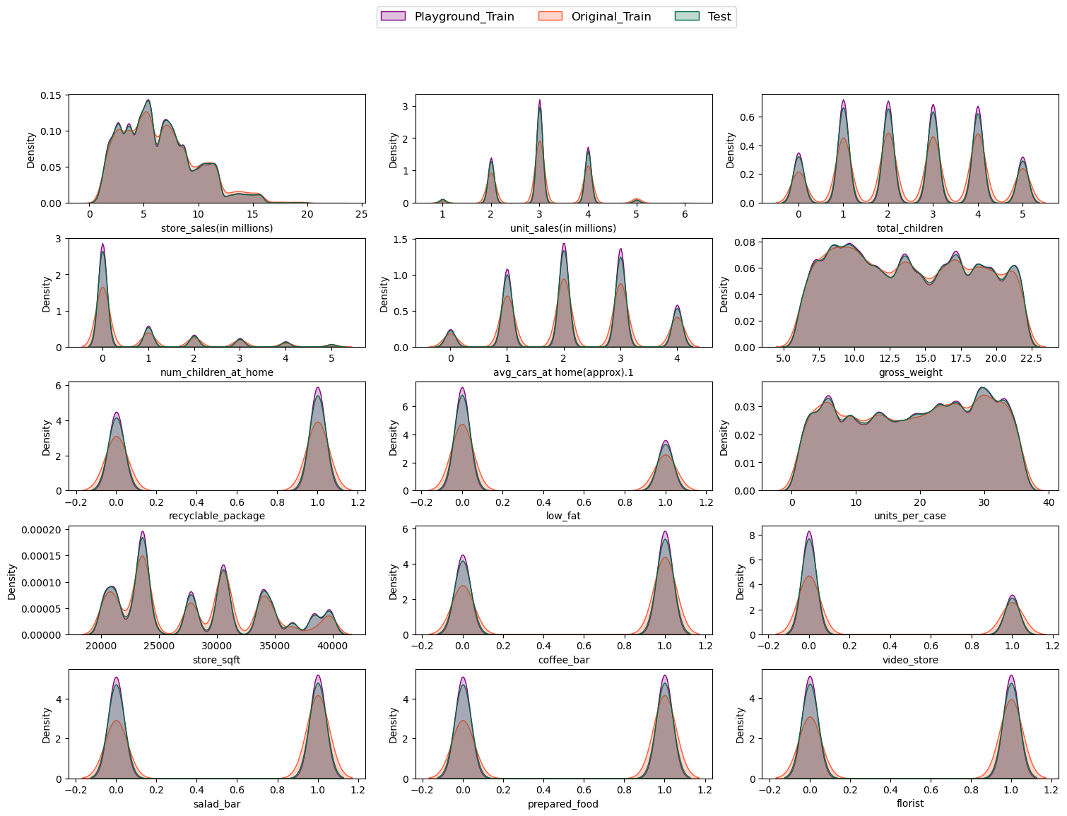
根据分布操场和原始训练集的趋势,将它们结合在一起似乎是合乎逻辑的,这在问题的描述中也有建议。
训练数据集和测试数据集中不同特征的比较描述了一个相同的分布。
连续和分类的特征可以被识别。
这些特征是二进制的:可回收包装,低脂肪,咖啡店,视频店,沙拉店,熟食店,花店。
这些特征有5-6个不同的值,可以被视为分类的:单位销售额(百万),儿童总数,在家的儿童数量,在家的平均汽车数量(大约)。
我们得到了4个连续特征:商店销售额(百万)、总重量、每箱单位、商店面积。
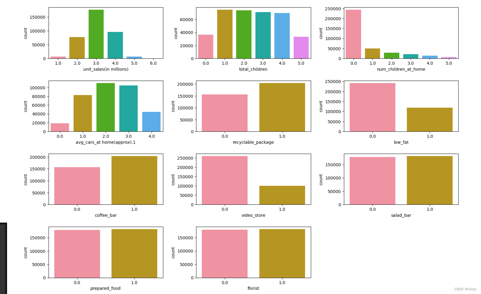
3.2 Categorical and Continues distribution
Lets asses the distribution of categorical features in the train database closely.
In [10]:
linkcode
Continuous = ["store_sales(in millions)", "gross_weight", "units_per_case", "store_sqft"]
binary = ["recyclable_package", "low_fat", "coffee_bar", "video_store", "salad_bar", "prepared_food", "florist"]
categorical = ["unit_sales(in millions)", "total_children", "num_children_at_home", "avg_cars_at home(approx).1"]
categorical.extend(binary)

# Create a custom HUSL color palette with a different color
colors = sns.husl_palette(n_colors=6, s=1.0, l=0.7)

# Create multiple plots with a gicven size
fig = plt.figure(figsize=(15,10))


# Create a countplot to evaluate the distribution
for i, cat_feature in enumerate(categorical):
    ax = plt.subplot(4, 3, i+1)
    sns.countplot(x=cat_feature, data=P_train_df, palette=colors, ax=ax)

# Fitting the labels for each plot
fig.tight_layout(pad=2)
编辑
数据集在沙拉店、熟食店、花店方面的分布是均匀的。
然而,咖啡吧和可回收包装则被认为是最多存在的。
此外,视频商店、低脂食品在数据集中似乎更有可能为零。
Unit_sales第6类不能真正被识别。
根据sergiosaharovskiy的说法,salad_bar和prepared_food几乎是一样的,删除其中一个可能是好的。
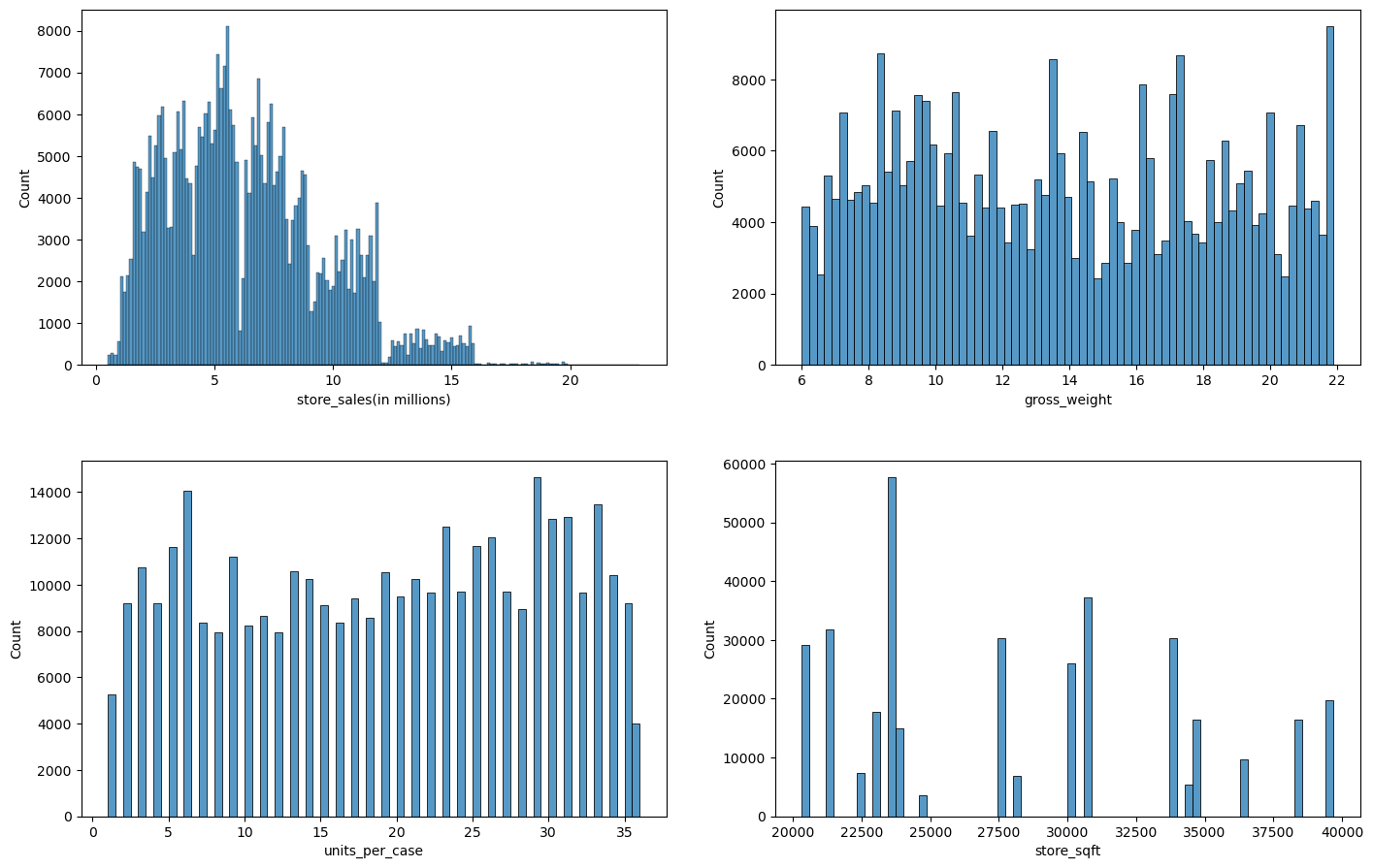
在评估了分类特征的分布后,我们可以用直方图研究连续特征:
# Create multiple plots
fig, axes = plt.subplots(nrows=2, ncols=2, figsize=(15,10))
fig.tight_layout(pad=5)

# Create a countplot to evaluate the distribution
for i, num_feature in enumerate(Continuous):
    row = i // 2
    col = i % 2
    ax = axes[row, col]
    sns.histplot(x=num_feature, data=P_train_df, ax=ax)
编辑
考虑到商店销售额的变化(以百万计),我们可以解释说,我们的大部分数据是在500万商店销售额左右,随着它的增加,我们的数据开始减少了。
另一方面,总重量和每箱单位的分布似乎是均匀的。
此外,store_sqft代表大多数可用的数据大约是22500平方英尺。
store_sqft特征只得到了20个不同的值,而units_per_case特征只得到了30个不同的值。
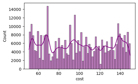
3.3 目标变量分布
对目标值的分布进行了研究,看看它的影响,看看目标有多少个独特的值。@Janmpia笔记本建议,这个问题似乎不是一个回归问题,因为有训练数据集的目标值,但测试集的目标值是未知的,因此,把它看作是一个分类问题似乎是一个冒险的做法。这种复杂情况可能是由于数据集的合成性质造成的。
target_col = "cost"

# Calculate the unique values, median, mean, and mode of the target variable
unique_values = len(P_train_df[target_col].unique())
maximum = P_train_df[target_col].max()
minimum = P_train_df[target_col].min()
median = P_train_df[target_col].median()
mean = P_train_df[target_col].mean()
mode = P_train_df[target_col].mode().values[0]

print(f'''
Target variable description
Number of unique_values = {unique_values}
Maximum = {maximum}
Minimum = {minimum}
Median = {median}
Mean = {mean}
Mode = {mode}
''')
Target variable description
Number of unique_values = 328
Maximum = 149.75
Minimum = 50.79
Median = 98.81
Mean = 99.61472939145688
Mode = 101.84
In [13]:
fig = plt.figure(figsize=(5,3))
sns.histplot(data=P_train_df, x="cost", kde=True, color='purple', alpha=0.5)
Out[13]:
<AxesSubplot:xlabel='cost', ylabel='Count'>
编辑
从成本的分布来看,我们了解到分布是偏斜的,有多个峰值和谷值,目标变量中没有离群值。
在这种情况下,分布中存在多个局部最大值和最小值,可能表明影响结果的因素以复杂的方式相互作用。
成本有大约328个独特的值,这意味着目标在某种程度上是连续的。
矩阵的相关性:(略):
Salad_bar和prepared_food似乎是相同的,它们之间存在着完美的相关性,所以删除其中一个是合理的。
正如前面提到的,原始训练集和操场训练集的相关矩阵表明了相同的模式,因此将它们结合起来是合理的。
所有的特征似乎都有很低的相关系数,因此它们不能单独解释成本。
DATA:
4.1 Combine Origina and Playground
train_df = pd.concat([P_train_df, O_train_df], axis=0)
# remove id and prepared food
train_df.drop(columns=["id","prepared_food"], inplace=True)

# removing unit 6 from unit_sales(in millions)
train_df['unit_sales(in millions)'] = train_df['unit_sales(in millions)'].replace(6.0, 5.0)
P_test_df['unit_sales(in millions)'] = P_test_df['unit_sales(in millions)'].replace(6.0, 5.0)

train_df.tail()
4.2 Feature selection
selected_features = [
 'total_children',
 'num_children_at_home',
 'avg_cars_at home(approx).1',
 'store_sqft',
 'coffee_bar',
 'video_store',
 'salad_bar',
 'florist',
]
4.3 Feature engineering
def feature_eng(df):
    # Ratio of children at home to total_children
    df['children_per_adult']= df["num_children_at_home"] / df["total_children"]
    df['children_per_adult'].replace([np.inf, -np.inf], 10, inplace=True)
    df['children_per_adult'].fillna(0, inplace = True)

    # Weight per unit
    df["weight_per_unit"] = df["gross_weight"] / df["unit_sales(in millions)"]
    df['weight_per_unit'].replace([np.inf, -np.inf, np.nan], 0, inplace=True)

    # Num of units sold per area
    df["Units_per_area"] = df["unit_sales(in millions)"] / df["store_sqft"]
    df['Units_per_area'].replace([np.inf, -np.inf, np.nan], 0, inplace=True)

    # sales per unit
    df['sales_per_unit'] = df["store_sales(in millions)"] / df["unit_sales(in millions)"]
    df['sales_per_unit'].replace([np.inf, -np.inf, np.nan], 0, inplace=True)

    # sales_per_unit_weight
    df['sales_per_unit_weight'] = df["store_sales(in millions)"] / df["gross_weight"]
    df['sales_per_unit_weight'].replace([np.inf, -np.inf, np.nan], 0, inplace=True)

    # Sales per area of the shop
    df['sales_per_area'] = df["store_sales(in millions)"] / df["store_sqft"]
    df['sales_per_area'].replace([np.inf, -np.inf, np.nan], 0, inplace=True)

    # Presence of any amenities
    df[['coffee_bar', 'video_store', 'low_fat', 'salad_bar', 'florist']] = df[['coffee_bar', 'video_store', 'low_fat', 'salad_bar', 'florist']].astype(int)

    df['any_amenities'] = df[['coffee_bar', 'video_store', 'salad_bar', 'florist']].any(axis=1)

    # Num of independent_children
    df['independent_children'] = df['total_children'] - df['num_children_at_home']
    df['independent_children'].replace([np.inf, -np.inf, np.nan], 0, inplace=True)

    # Create a new feature for child-to-car ratio
    # the transportation needs of households with children
    df['child_to_car_ratio'] = df['total_children'] / df['avg_cars_at home(approx).1']
    df['child_to_car_ratio'].replace([np.inf, -np.inf], 10, inplace=True)
    df['child_to_car_ratio'].fillna(0, inplace = True)

    # Create a new feature for healthy food options
    df['healthy_food_options'] = df['low_fat'] & df['salad_bar']

    # Create a new feature for customer age group
    df['customer_age_group'] = df['total_children'] / df['num_children_at_home']
    df['customer_age_group'].replace([np.inf, -np.inf], 10, inplace=True)
    df['customer_age_group'].fillna(0, inplace = True)

    # Percentage of low-fat items
    # df['pct_low_fat'] = (df['low_fat'].sum() / df['unit_sales(in millions)'].sum()) * 100
    # df['pct_low_fat'] = df['low_fat'].replace(np.nan, 0).replace(np.inf, 0) / pct_low_fat
    return df
检查略
4.4 Define X & y
In [24]:
# Define a function to find X and y arrays for a given dataframe either test or train
def getXy(df,X_label=None,y_label=None,cat_label=None):
    # cases that X_label is not given and it is all the features except target
    if X_label is None:
        X = df[[c for c in df.columns if c!=y_label]].values
    else:
        # Change the X array to one column when there is only one X_label
        if len(X_label) == 1:
            X = df[X_label].values.reshape(-1,1)
        else:
            # Find X based on the given X_labels when there are multiple X_labels
            X = df[X_label].values
    if y_label is None:
        # Create a zero array in the case of test set which we dont want the y_test
        y = np.zeros(df.shape[0]).reshape(-1,1)
    else:
        # calc target value and reshape it in a single column
#         y = df[y_label].values.reshape(-1,1)
        y = df[y_label].values
    # Feature Scaling
#     scaler = StandardScaler()
#     X = scaler.fit_transform(X)

    # Use One Hot encoding for categorical features
    if cat_label is None:
        # create a new dataframe with X and Y
        label = np.hstack((X_label,y_label))
        data = pd.DataFrame(np.hstack((X,y.reshape(-1,1))), columns=label)
    else:
        data = pd.get_dummies(df, columns = cat_label)
    return data,X, y
In [25]:
# Scale the store_sqft column using MinMaxScaler
scaler = MinMaxScaler()
train_df['store_sqft'] = scaler.fit_transform(train_df[['store_sqft']])
P_test_df['store_sqft'] = scaler.fit_transform(P_test_df[['store_sqft']])
In [26]:
# engineer_labels = ['children_per_adult', 'weight_per_unit', 'Units_per_area', 'sales_per_unit',
#                    'sales_per_unit_weight', 'sales_per_area', 'any_amenities', 'independent_children',
#                    'child_to_car_ratio','healthy_food_options', 'customer_age_group']
engineer_labels = ['children_per_adult','independent_children','customer_age_group','any_amenities','child_to_car_ratio']
# engineer_labels = []
selected_features.extend(engineer_labels)
print(selected_features)
['total_children', 'num_children_at_home', 'avg_cars_at home(approx).1', 'store_sqft', 'coffee_bar', 'video_store', 'salad_bar', 'florist', 'children_per_adult', 'independent_children', 'customer_age_group', 'any_amenities', 'child_to_car_ratio']
In [27]:
names = list(P_train_df.columns)
item_to_remove=['id','prepared_food','recyclable_package','store_sales(in millions)','units_per_case',
                'low_fat','gross_weight','unit_sales(in millions)','cost']
for i in item_to_remove:
    names.remove(i)
names.extend(engineer_labels)
features = [c for c in names if c!="cost"]
print(names)
['total_children', 'num_children_at_home', 'avg_cars_at home(approx).1', 'store_sqft', 'coffee_bar', 'video_store', 'salad_bar', 'florist', 'children_per_adult', 'independent_children', 'customer_age_group', 'any_amenities', 'child_to_car_ratio']
In [28]:
train,X,y = getXy(train_df,X_label=names,y_label="cost")
print(X.shape)
print(y.shape)
(411699, 13)
(411699,)
In [29]:
test,X_,y_ = getXy(P_test_df,X_label=names)
print(X_.shape)
print(y_.shape)
(240224, 13)
(240224, 1)
之后预测即可:
随机森林回归器显示RMSLE的预测值较低
将CatBoost与随机森林回归器混合使用似乎是个好主意。
- store_sqft seems to be more significant.
6. Model tuning
Due to the large computational cost of randome forest regressor model Xgboost was chosen to tune.
In [49]:
from sklearn.model_selection import KFold

xgb_param= {'n_estimators': 100, # not imp
             'learning_rate': 0.95, # + or - bad
             'max_depth': 15, # - bad + bad
             'lambda': 0.0150, # + bad
             'alpha': 1.0e-08, # - is little good
             'colsample_bytree': 0.7, # imp (adding randomness to the training process.)
             'min_child_weight': 0, # + bad
             'booster': 'gbtree',
             'grow_policy': 'depthwise',
             'tree_method': 'gpu_hist',
             'gpu_id': 0,
             'objective': 'reg:squaredlogerror',
             'eval_metric': 'rmsle',
             'early_stopping_rounds': 10.0, # not imp
             'random_state': 17}

tune_xgb_reg = XGBRegressor(**xgb_param)

# Define the K-fold cross-validation generator
cv = KFold(n_splits=5, shuffle=True, random_state=17)

# Perform cross-validation
scores = []
for fold_idx, (train_idx, test_idx) in enumerate(cv.split(X)):
    # Get the training and test sets
    X_train, X_test = X[train_idx], X[test_idx]
    y_train, y_test = y[train_idx], y[test_idx]

    # Train the model with early stopping
    tune_xgb_reg.fit(X_train, y_train, eval_set=[(X_test, y_test)], verbose=False)

    # Make predictions on the test set
    y_pred = tune_xgb_reg.predict(X_test)

    # Compute the root mean squared log error
    score = rmsle(y_test, y_pred)
    scores.append(score)
    # Print the score for this fold
    print(f'Fold {fold_idx+1}: root mean squared log error = {score:.4f}')
# Compute the mean score across all folds
mean_score = sum(scores) / len(scores)
print(f'Mean root mean squared log error across {cv.n_splits} folds: {mean_score:.4f}')
RMSLE.append(rmsle(y_test,y_pred))
print(RMSLE)
Fold 1: root mean squared log error = 0.2933
Fold 2: root mean squared log error = 0.2937
Fold 3: root mean squared log error = 0.2939
Fold 4: root mean squared log error = 0.2938
Fold 5: root mean squared log error = 0.2933
Mean root mean squared log error across 5 folds: 0.2936
[0.293268473999593]
7. Submission
In [50]:
linkcode
y_sub = tune_xgb_reg.predict(X_)
Export = np.hstack((np.reshape(P_test_df["id"].values, (-1,1)), np.reshape(y_sub, (-1,1))))
Submission = pd.DataFrame(Export, columns=["id", "cost"])
Submission.to_csv(r'submission.csv', index=False, header=["id", "cost"])

 浙公网安备 33010602011771号