Reinforcement Learning: From Fundamentals to GRPO Algorithm

Reinforcement Learning: From Fundamentals to GRPO Algorithm

This lecture will guide you through the core concepts of reinforcement learning, starting from the basics and progressively delving into advanced algorithms such as PPO and GRPO.

1. Overview of Reinforcement Learning

• Goal: The primary objective of RL is for an agent to learn a policy (\(\pi\)) that maximizes the expected cumulative reward (return) through interaction with a dynamic environment.
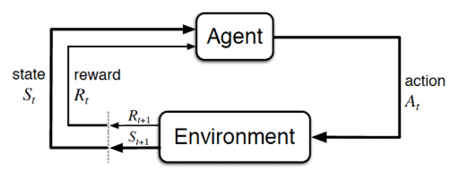
• Core Components:
  • Agent: The learner or decision-maker.
  • Environment: Everything external to the agent, defining the world the agent operates in.
  • State (\(S_t\)): A representation of the environment at time \(t\).
  • Action (\(A_t\)): The choice made by the agent at time \(t\).
  • Reward (\(R_{t+1}\)): A scalar feedback signal received by the agent from the environment after executing an action in a state, indicating the immediate "goodness" of that action.
  • Trajectory (\(\tau\)): A complete sequence of state-action-reward transitions: \(\tau = (S_0, A_0, R_1, S_1, A_1, R_2, \dots, S_T)\)
• Example: Frozen Lake game
  

1.1 Markov Decision Process (MDP)

Reinforcement learning problems are typically formalized as Markov Decision Processes (MDPs).
An MDP is defined by the following elements:

• A set of states \(\mathcal{S}\).
• A set of actions \(\mathcal{A}\).
• A state transition probability function \(P(s'|s, a) = P(S_{t+1}=s' | S_t=s, A_t=a)\), representing the probability of transitioning to state \(s'\) after taking action \(a\) in state \(s\).
• A reward function \(\mathcal{R}(s, a, s')\), representing the expected reward received after taking action \(a\) in state \(s\) and transitioning to state \(s'\). Sometimes simplified to \(\mathcal{R}(s,a)\) or \(\mathcal{R}(s)\).

A key assumption of MDPs is the Markov Property: The future depends only on the current state and action, independent of the past.

\[P(S_{t+1}|S_t, A_t, S_{t-1}, A_{t-1}, \dots, S_0, A_0) = P(S_{t+1}|S_t, A_t) \]

1.2 Policy (\(\pi\))

The policy (\(\pi\)) defines the agent's behavior at a given time. It is a mapping from environment states to actions.

• Deterministic Policy: \(a = \pi(s)\)
• Stochastic Policy: \(\pi(a|s) = P(A_t=a | S_t=s)\)

The ultimate goal is to find an optimal policy (\(\pi_*\)) that maximizes the expected cumulative reward.

\[\pi_* = \arg\max_{\pi} \mathbb{E} \left[ \sum_{k=0}^{\infty} \gamma^k R_{t+k+1} \right] \]

(The expectation is based on trajectories starting from some initial state under policy \(\pi\).)

2. Value Functions and Bellman Equations

To evaluate the "goodness" of a state or an action, we introduce value functions.

2.1 Return \(G_t\)

The return (\(G_t\)) is the total discounted reward starting from time step \(t\).

\[G_t = R_{t+1} + \gamma R_{t+2} + \gamma^2 R_{t+3} + \dots = \sum_{k=0}^{\infty} \gamma^k R_{t+k+1} \]

where \(\gamma \in [0, 1]\) is the discount factor, balancing the importance of immediate versus future rewards.
Recursive relation:

\[G_t = R_{t+1} + \gamma G_{t+1} \]

2.2 State-Value Function \(V_\pi(s)\)

The state-value function (\(V_\pi(s)\)) represents the expected return starting from state \(s\), and thereafter following policy \(\pi\).

\[V_\pi(s) = \mathbb{E}_\pi [G_t | S_t=s] \]

It quantifies the "goodness" of being in a particular state \(s\) under policy \(\pi\).

2.3 Action-Value Function \(Q_\pi(s,a)\)

The action-value function (\(Q_\pi(s,a)\)) represents the expected return after taking action \(a\) in state \(s\), and thereafter following policy \(\pi\).

\[Q_\pi(s,a) = \mathbb{E}_\pi [G_t | S_t=s, A_t=a] \]

It quantifies the "goodness" of taking a specific action \(a\) in state \(s\) under policy \(\pi\).

2.4 Relationship between \(V_\pi(s)\) and \(Q_\pi(s,a)\)

\[V_\pi(s) = \sum_{a \in \mathcal{A}} \pi(a|s) Q_\pi(s,a) \]

This means the value of a state is the expected value of all possible actions in that state, weighted by the probability of the policy selecting each action.

2.5 Bellman Equations

Bellman Equations define the recursive relationships of value functions and are the cornerstone of reinforcement learning.

• Bellman Expectation Equation for \(V_\pi(s)\):

  \[V_\pi(s) = \mathbb{E}_\pi [R_{t+1} + \gamma V_\pi(S_{t+1}) | S_t=s] \]
  \[V_\pi(s) = \sum_{a \in \mathcal{A}} \pi(a|s) \left( \mathcal{R}(s,a) + \gamma \sum_{s' \in \mathcal{S}} P(s'|s, a) V_\pi(s') \right) \]

• Bellman Expectation Equation for \(Q_\pi(s,a)\):

  \[Q_\pi(s,a) = \mathbb{E}_\pi [R_{t+1} + \gamma Q_\pi(S_{t+1}, A_{t+1}) | S_t=s, A_t=a] \]
  \[Q_\pi(s,a) = \mathcal{R}(s,a) + \gamma \sum_{s' \in \mathcal{S}} P(s'|s, a) \sum_{a' \in \mathcal{A}} \pi(a'|s') Q_\pi(s',a') \]

Relationship:

2.6 Optimal Value Functions

The optimal state-value function \(V_*(s)\) is the maximum expected return achievable from state \(s\).

\[V_*(s) = \max_{\pi} V_\pi(s) \]

The optimal action-value function \(Q_*(s,a)\) is the maximum expected return achievable after taking action \(a\) in state \(s\) and thereafter following an optimal policy.

\[Q_*(s,a) = \max_{\pi} Q_\pi(s,a) \]

2.7 Bellman Optimality Equations

Policy \(\pi^*\) is optimal if and only if for all states \(s\), its state-value function is not smaller than the value function of any other policy:

\[V^{\pi^*}(s) \geq V^\pi(s) \quad \forall s \in \mathcal{S}, \forall \pi \]

that is:

\[\pi^* = \arg\max_{\pi} V^\pi(s) \quad \forall s \]

The Bellman Optimality Equations describe the value functions corresponding to the optimal policy \(\pi_*\).

• For \(V_*(s)\):
  \[V_*(s) = \max_{a \in \mathcal{A}} \left( \mathcal{R}(s,a) + \gamma \sum_{s' \in \mathcal{S}} P(s'|s, a) V_*(s') \right) \]

• For \(Q_*(s,a)\):
  \[Q_*(s,a) = \mathcal{R}(s,a) + \gamma \sum_{s' \in \mathcal{S}} P(s'|s, a) \max_{a' \in \mathcal{A}} Q_*(s',a') \]

• Property: \(\pi_*\) exists and can be solved for.

3. Solving/Estimating Value Functions

• Closed-form solution

\[r_{\pi}(s)\doteq\sum_{a\in\mathcal{A}}\pi(a|s)\sum_{r\in\mathcal{R}}p(r|s,a)r \]

\[p_{\pi}(s'|s)\doteq\sum_{a\in\mathcal{A}}\pi(a|s)p(s'|s,a) \]

\[v_{\pi}(s)=r_{\pi}(s)+\gamma\sum_{s'\in\mathcal{S}}p_{\pi}(s'|s)v_{\pi}(s') \]

\[\underbrace{\begin{bmatrix}v_{\pi}(s_1)\\v_{\pi}(s_2)\\v_{\pi}(s_3)\\v_{\pi}(s_4)\end{bmatrix}}_{v_{\pi}}=\underbrace{\begin{bmatrix}r_{\pi}(s_1)\\r_{\pi}(s_2)\\r_{\pi}(s_3)\\r_{\pi}(s_4)\end{bmatrix}}_{r_{\pi}}+\gamma\underbrace{\begin{bmatrix}p_{\pi}(s_1|s_1)&p_{\pi}(s_2|s_1)&p_{\pi}(s_3|s_1)&p_{\pi}(s_4|s_1)\\p_{\pi}(s_1|s_2)&p_{\pi}(s_2|s_2)&p_{\pi}(s_3|s_2)&p_{\pi}(s_4|s_2)\\p_{\pi}(s_1|s_3)&p_{\pi}(s_2|s_3)&p_{\pi}(s_3|s_3)&p_{\pi}(s_4|s_3)\\p_{\pi}(s_1|s_4)&p_{\pi}(s_2|s_4)&p_{\pi}(s_3|s_4)&p_{\pi}(s_4|s_4)\end{bmatrix}}_{P_{\pi}}\underbrace{\begin{bmatrix}v_{\pi}(s_1)\\v_{\pi}(s_2)\\v_{\pi}(s_3)\\v_{\pi}(s_4)\end{bmatrix}}_{v_{\pi}} \]

\[v_{\pi}=r_{\pi}+\gamma P_{\pi}v_{\pi} \]

Solution:

\[v_{\pi}=(I - \gamma P_{\pi})^{-1}r_{\pi} \]

• Iteration solution

For large state spaces, directly solving the Bellman equations is computationally expensive.

\[v_{k + 1} = r_{\pi}+\gamma P_{\pi}v_{k}, \quad k = 0,1,2,\ldots \]

This algorithm generates a sequence of values \(\{v_0, v_1, v_2, \ldots\}\), where \(v_0\in\mathbb{R}^n\) is an initial guess of \(v_{\pi}\).

It holds that

\[v_{k} \to v_{\pi} = (I - \gamma P_{\pi})^{-1}r_{\pi}, \quad \text{as } k\to\infty \]

This is actually a dynamic programming (DP) idea.

• Assumes the environment model (i.e., \(P\) and \(\mathcal{R}\)) is known.
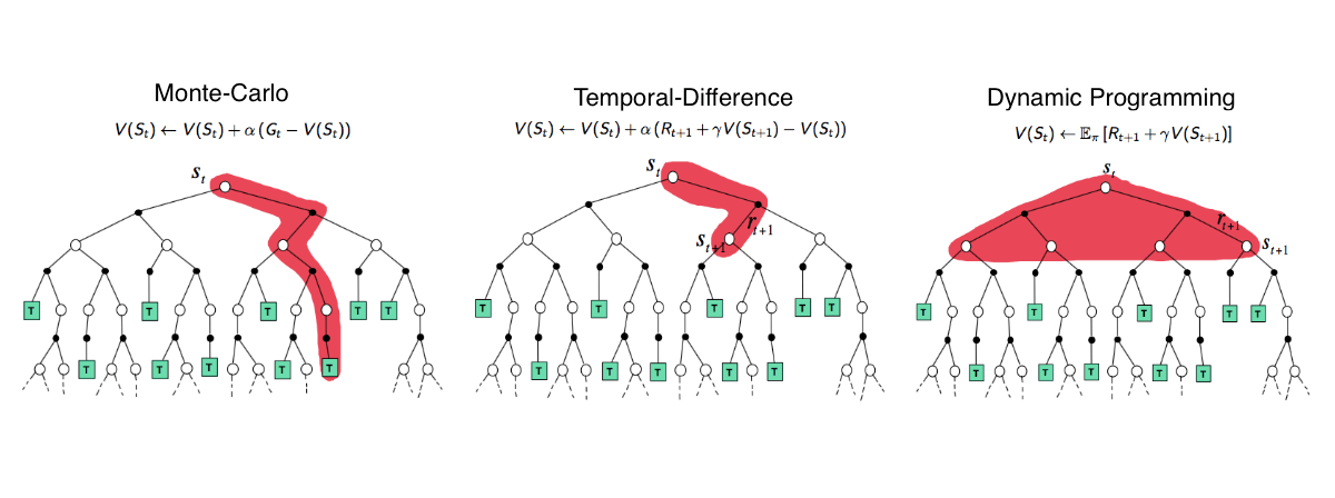
• Update rule: \(V(S_t) \leftarrow \mathbb{E}_\pi[R_{t+1} + \gamma V(S_{t+1}) | S_t=S_t]\).

Two methods for estimating value functions when the model is unknown:

• Monte Carlo (MC)

  • Learns directly from complete experience episodes without an environment model (model-free).
  • Estimates the value function by averaging the returns observed after visiting a state.
  • \(V_\pi(s) \approx \frac{1}{N}\sum_{i=1}^{N}G_t^{(i)}\), where \(G_t^{(i)}\) is the return starting from state \(s\) in the \(i\)-th episode.
  • MC methods only update the value of a state after the completion of an episode.
  • Update rule: \(V(S_t) \leftarrow V(S_t) + \alpha (G_t - V(S_t))\), where \(\alpha\) is the learning rate.

• Temporal Difference (TD)

  • Also model-free, learns from experience.
  • Updates value estimates based on other learned estimates without waiting for a final outcome (bootstrapping).
  • The simplest TD method, TD(0), uses the observed reward \(R_{t+1}\) and the estimated value of the next state \(S_{t+1}\) to update the value of \(S_t\).
  • Update rule: \(V(S_t) \leftarrow V(S_t) + \alpha (R_{t+1} + \gamma V(S_{t+1}) - V(S_t))\).
    • The term \(R_{t+1} + \gamma V(S_{t+1}) - V(S_t)\) is called the TD error.

4. Model-Based RL

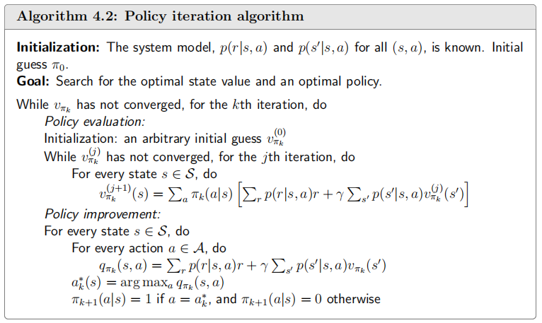
4.1 Policy Iteration

Two alternating phases:

1. Policy Evaluation: Given a policy \(\pi\), compute its state-value function \(V_\pi\).
2. Policy Improvement: Greedily improve the policy based on \(V_\pi\). For each state \(s\), select the action \(a\) that maximizes \(Q_\pi(s,a)\).
   \[\pi'(s) = \arg\max_a Q_\pi(s,a) = \arg\max_a \left( \mathcal{R}(s,a) + \gamma \sum_{s'} P(s'|s, a) V_\pi(s') \right) \]

Repeat this process until the policy converges to the optimal policy \(\pi_*\).

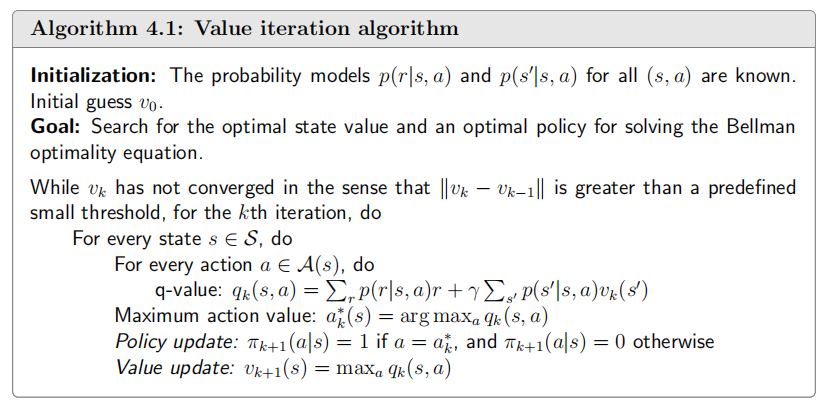
4.2 Value Iteration

Value iteration merges partial policy evaluation and improvement into a single update step. It directly iteratively applies the Bellman optimality equation to find \(V_*\).

\[V_{k+1}(s) = \max_{a \in \mathcal{A}} \left( \mathcal{R}(s,a) + \gamma \sum_{s' \in \mathcal{S}} P(s'|s, a) V_k(s') \right) \]

Because the Bellman optimality operator is a contraction mapping, value iteration is guaranteed to converge to \(V_*\). Once \(V_*\) is found, the optimal policy can be extracted by selecting actions that maximize the expected return under \(V_*\).

5. Value-Based RL

When the environment model (state transition probabilities \(P\) and rewards \(\mathcal{R}\)) is unknown, we use model-free RL methods. These methods learn the optimal policy by interacting with the environment and collecting samples.

Classification:

• Value-Based RL: Learns a value function that maps states (or state-action pairs) to values, then derives a policy from these values (e.g., greedy selection).
• Policy-Based RL: Directly learns the parameters of the policy, not necessarily requiring a value function.
• Actor-Critic Methods: Combine features of both, learning a policy (actor) and a value function (critic) simultaneously.

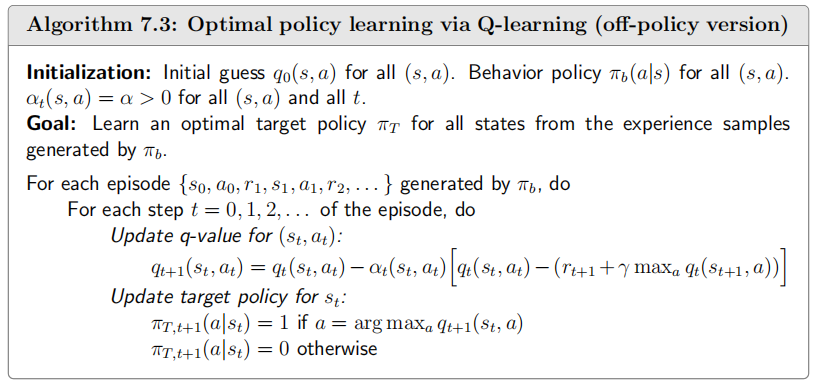
5.1 Q-learning (Off-Policy TD Control)

Q-learning is an off-policy TD control algorithm. Off-policy means the policy being learned (the target policy, the optimal greedy policy) is different from the policy used to generate behavior (the behavior policy, which can be more exploratory).

• Goal: Directly learn the optimal action-value function \(Q_*(s,a)\).
• It aims to solve the Bellman optimality equation for \(Q_*(s,a)\):
  \[Q_*(s,a) = \mathbb{E}[R_{t+1} + \gamma \max_{a'} Q_*(S_{t+1}, a') | S_t=s, A_t=a] \]

• Update Rule:
  For a transition \((s_t, a_t, r_{t+1}, s_{t+1})\):
  \[Q(s_t, a_t) \leftarrow Q(s_t, a_t) + \alpha \left[ r_{t+1} + \gamma \max_{a' \in \mathcal{A}} Q(s_{t+1}, a') - Q(s_t, a_t) \right] \]
  The agent uses the action \(a_t\) generated by its behavior policy, but the update incorporates the maximum Q-value for the next state \(s_{t+1}\), effectively learning about the greedy (optimal) policy. Once \((s_t, a_t)\) is given, the reward \(r_{t+1}\) and next state \(s_{t+1}\) do not depend on any specific policy.

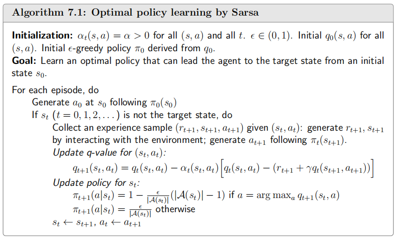
5.2 SARSA (On-Policy TD Control)

SARSA is an on-policy TD control algorithm. On-policy means it learns the value function for the same policy currently being used for decision-making.

• Goal: Learn the action-value function \(Q_\pi(s,a)\) for the current behavior policy \(\pi\).
• It aims to solve the Bellman equation for \(Q_\pi(s,a)\) under the current policy \(\pi\):
  \[Q_\pi(s,a) = \mathbb{E}[R_{t+1} + \gamma Q_\pi(S_{t+1}, A_{t+1}) | S_t=s, A_t=a] \]
  where \(A_{t+1} \sim \pi(A_{t+1}|S_{t+1})\).
• Update Rule:
  For a transition sequence \((s_t, a_t, r_{t+1}, s_{t+1}, a_{t+1})\) (the origin of the name SARSA):
  \[Q(s_t, a_t) \leftarrow Q(s_t, a_t) + \alpha \left[ r_{t+1} + \gamma Q(s_{t+1}, a_{t+1}) - Q(s_t, a_t) \right] \]
  Here, \(a_{t+1}\) is the action actually taken in state \(s_{t+1}\) according to the current policy \(\pi\). The target policy and the behavior policy are identical.

6. Entering the Deep Learning Era

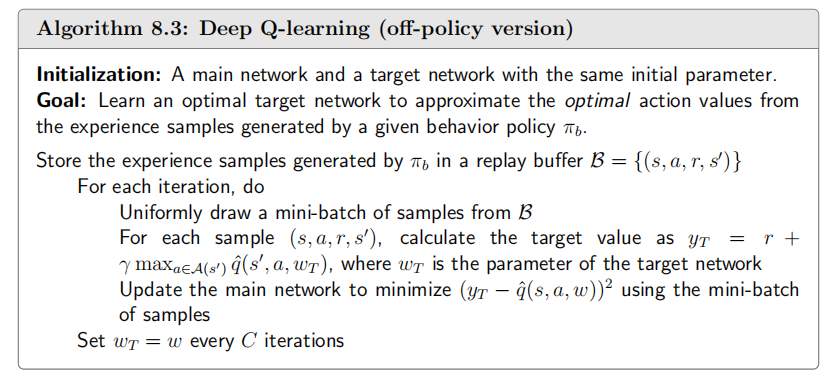
6.1 Function Approximation

Tabular reinforcement learning can only represent a limited number of discrete states, whereas real-world scenarios often involve continuous states. Neural networks can be used to represent value functions and policies.

6.2 DQN (Deep Q-Network)

7. Policy Gradient Methods

Policy gradient methods do not learn a value function and then derive a policy. Instead, they directly parameterize the policy \(\pi(a|s, \theta)\) (with parameters \(\theta\)) and optimize these parameters by performing gradient ascent on an objective function \(J(\theta)\).

7.1 Objective Function

The objective function \(J(\theta)\) quantifies the policy's performance. Common choices include:

• Average State Value: \(J(\theta) = \sum_{s} d^{\pi}(s) v^{\pi}(s)\)
• Average Reward: \(J(\theta) = \lim_{T \to \infty} \frac{1}{T} \mathbb{E}\left[\sum_{t=0}^{T-1} R_t \right]\)
• Start-State Value (episodic tasks): \(J(\theta) = v^{\pi}(s_0)\)

Here \(d^{\pi}(s)\) is the stationary state distribution under \(\pi\), and \(v^{\pi}(s)\) is the state-value function. The choice depends on the problem structure (continuing vs. episodic tasks).

7.2 Policy Gradient Theorem

The Policy Gradient Theorem provides an analytical expression for \(\nabla_\theta J(\theta)\) that avoids differentiating through state distributions. For any differentiable policy \(\pi(a|s,\theta)\), the gradient is:

\[\nabla_{\theta} J(\theta) = \sum_{s \in \mathcal{S}} \eta(s) \sum_{a \in \mathcal{A}} \nabla_{\theta} \pi(a | s, \theta) q_{\pi}(s, a) \]

where \(\eta(s)\) is the state distribution (stationary \(d^\pi(s)\) or discounted), and \(q_{\pi}(s, a)\) is the action-value function. Applying the log-derivative trick \(\nabla_\theta \pi = \pi \nabla_\theta \ln \pi\), we derive equivalent forms:

\[\begin{aligned} \nabla_{\theta} J(\theta) & = \sum_{s} \eta(s) \sum_{a} \pi(a | s, \theta) \nabla_{\theta} \ln \pi(a | s, \theta) q_{\pi}(s, a) \\ & = \mathbb{E}_{S \sim \eta}\left[\sum_{a} \pi(a | S, \theta) \nabla_{\theta} \ln \pi(a | S, \theta) q_{\pi}(S, a)\right] \\ & = \mathbb{E}_{S \sim \eta, A \sim \pi}\left[\nabla_{\theta} \ln \pi(A | S, \theta) q_{\pi}(S, A)\right] \end{aligned} \]

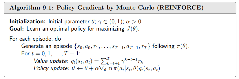
7.3 REINFORCE (Monte Carlo Policy Gradient)

REINFORCE is a fundamental Monte Carlo policy gradient algorithm.

• Updates policy parameters \(\theta\) in the direction of \(\nabla_\theta J(\theta)\).
• Uses the complete cumulative return \(G_t\) as an unbiased estimate of \(q_{\pi_\theta}(s_t, a_t)\).
• Algorithm Steps:

Policy gradient methods can suffer from high variance in gradient estimates, leading to slow convergence.

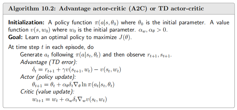
8. Actor-Critic Methods

8.1 Baselines

To reduce variance, a baseline (\(b(s)\)) can be subtracted from the return/Q-value in the policy gradient expression. A baseline is any function that does not depend on the action \(a\). A common choice is the state-value function \(V_{\pi_\theta}(s)\).

\[\nabla_\theta J(\theta) = \mathbb{E}_{S \sim \eta, A \sim \pi} \left[ \nabla_\theta \ln \pi_\theta(a|s) (Q_{\pi_\theta}(s,a) - V_{\pi_\theta}(s)) \right] \]

The term \(A_{\pi_\theta}(s,a) = Q_{\pi_\theta}(s,a) - V_{\pi_\theta}(s)\) is called the Advantage Function.

• \(A_{\pi_\theta}(s,a)\) measures how much better taking action \(a\) in state \(s\) is compared to following the average action under policy \(\pi_\theta\).
• If \(A > 0\), increase the probability of taking action \(a\); if \(A < 0\), decrease it.
• The advantage function can be estimated, for example, using the TD error:
  \[A_{\pi_\theta}(s_t, a_t) \approx R_{t+1} + \gamma V_{\pi_\theta}(S_{t+1}) - V_{\pi_\theta}(S_t) \]
  This forms the basis of Actor-Critic methods, where the actor learns the policy and the critic learns the value function (or advantage function).

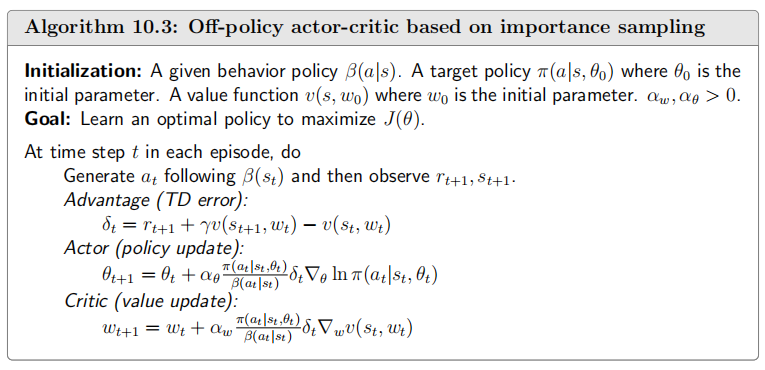
8.2 Importance Sampling

Importance sampling is a technique used to estimate the expectation of a function \(f(x)\) under a distribution \(p(x)\) by sampling from a different distribution \(q(x)\).

\[\mathbb{E}_{x \sim p}[f(x)] = \int f(x) p(x) dx = \int f(x) \frac{p(x)}{q(x)} q(x) dx = \mathbb{E}_{x \sim q}\left[f(x) \frac{p(x)}{q(x)}\right] \]

The term \(\frac{p(x)}{q(x)}\) is called the importance sampling ratio.
In RL, this allows us to evaluate a new policy \(\pi_\theta\) using data collected from an old policy \(\pi_{\theta_{old}}\) (off-policy learning), improving sample efficiency.
For the policy gradient objective function:

\[J(\theta) = \mathbb{E}_{s \sim d_{\pi_{\theta_{old}}}, a \sim \pi_{\theta_{old}}} \left[ \frac{\pi_\theta(a|s)}{\pi_{\theta_{old}}(a|s)} A_{\pi_{\theta_{old}}}(s,a) \right] \]

Then take the gradient of this expression.

However, large importance sampling ratios can lead to high variance.

8.3 Trust Region Policy Optimization (TRPO)

Traditional policy gradient methods can be unstable because a single bad update can drastically degrade policy performance. TRPO addresses this by constraining the magnitude of policy updates.

• Problem: Large policy updates can lead to performance collapse. The learning rate \(\alpha\) is difficult to choose.
• Solution: Maximize a surrogate objective function while constraining the change in the policy. The constraint is typically defined using the KL Divergence, which measures the difference between two probability distributions.
  • KL Divergence: \(D_{KL}(P||Q) = \sum_x P(x) \log \frac{P(x)}{Q(x)}\).
• TRPO Objective:
  \[\text{maximize}_\theta \quad \hat{\mathbb{E}}_t \left[ \frac{\pi_\theta(a_t|s_t)}{\pi_{\theta_{old}}(a_t|s_t)} \hat{A}_t \right]$$$$\text{subject to} \quad \hat{\mathbb{E}}_t [D_{KL}(\pi_{\theta_{old}}(\cdot|s_t) || \pi_\theta(\cdot|s_t))] \le \delta \]
  where \(\pi_{\theta_{old}}\) is the old policy, \(\hat{A}_t\) is the estimated advantage function, and \(\delta\) is the step size constraint.
  TRPO uses a second-order Taylor expansion of the objective and a linear approximation of the constraint, leading to a complex optimization problem often solved with the conjugate gradient algorithm.

8.4 Proximal Policy Optimization (PPO)

PPO aims to achieve the stability and reliability of TRPO with simpler implementation, first-order optimization, and better sample efficiency. It encompasses algorithms that also constrain policy updates.

Two main variants of PPO:

1. PPO-Penalty (Adaptive KL Penalty):

   \[\text{maximize}_\theta \quad \hat{\mathbb{E}}_t \left[ \frac{\pi_\theta(a_t|s_t)}{\pi_{\theta_{old}}(a_t|s_t)} \hat{A}_t - \beta D_{KL}(\pi_{\theta_{old}}(\cdot|s_t) || \pi_\theta(\cdot|s_t)) \right] \]

   Here, \(\beta\) is an adaptively adjusted coefficient. \(\beta\) is increased if the KL divergence is too high and decreased if it is too low.

2. PPO-Clip (Clipped Surrogate Objective): This is the more commonly used variant.
   Let \(r_t(\theta) = \frac{\pi_\theta(a_t|s_t)}{\pi_{\theta_{old}}(a_t|s_t)}\) be the probability ratio.
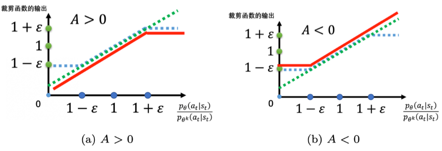
   The objective function is:

   \[L^{CLIP}(\theta) = \hat{\mathbb{E}}_t \left[ \min \left( r_t(\theta) \hat{A}_t, \quad \text{clip}(r_t(\theta), 1-\epsilon, 1+\epsilon) \hat{A}_t \right) \right] \]
   • \(\hat{A}_t\) is the estimator of the advantage function at time \(t\).
   • \(\epsilon\) is a small hyperparameter (e.g., 0.1 or 0.2) defining the clipping range.
   • The clip function restricts \(r_t(\theta)\) to the interval \([1-\epsilon, 1+\epsilon]\).
   • The \(\min\) operation takes the lesser of the unclipped objective \(r_t(\theta) \hat{A}_t\) and the clipped objective (a pessimistic bound).
     • If \(\hat{A}_t > 0\) (positive advantage, good action): The update is clipped when \(r_t(\theta)\) becomes too large (i.e., \(r_t(\theta) > 1+\epsilon\)), preventing overly aggressive policy updates.
     • If \(\hat{A}_t < 0\) (negative advantage, bad action): The update is clipped when \(r_t(\theta)\) becomes too small (i.e., \(r_t(\theta) < 1-\epsilon\)), preventing overly pessimistic updates (potentially reducing action probability too quickly).

   

Core Idea of PPO-Clip: Prevent large policy updates that move \(r_t(\theta)\) too far from 1 (i.e., make the new policy too different from the old policy) by clipping the objective function, leading to more stable learning. PPO typically performs multiple epochs of optimization on the same batch of sampled data.

Due to its good performance, ease of implementation, and tuning, PPO has become a preferred algorithm for many reinforcement learning applications.

8.5 Generalized Advantage Estimation (GAE)

The core idea of GAE is to combine TD errors from multiple time steps into a weighted sum, with weights controlled by \(\gamma\) and \(\lambda\). The standard GAE is defined as the discounted sum of all future TD errors:

\[A_t^{GAE(\gamma, \lambda)} = \sum_{l=0}^{\infty} (\gamma \lambda)^l \delta_{t+l} \]

where:

• \(\delta_{t+l} = R_{t+l} + \gamma V(s_{t+l+1}) - V(s_{t+l})\) is the TD error at time step \(t+l\).
• The summation starts from \(l=0\), meaning from the current time step \(t\) to the infinite future.
• \(\gamma\) is the discount factor (\(0 \leq \gamma \leq 1\)), adjusting the importance of future rewards.
• \(\lambda\) is the GAE parameter (\(0 \leq \lambda \leq 1\)), controlling the bias-variance tradeoff (\(\lambda = 0\) is low variance high bias, \(\lambda = 1\) is high variance low bias).
• \((\gamma \lambda)^l\) is the compound discount factor, combining \(\gamma\) (reward discounting) and \(\lambda\) (GAE tradeoff parameter).

This definition intuitively explains GAE: it's an exponentially weighted average of all future TD errors, with \(\lambda\) controlling the "horizon" of the estimate (larger \(\lambda\) relies on more future steps, increasing variance but decreasing bias).

Starting from the standard definition, we derive the recursive expression.

Expanding the standard definition:

\[A_t^{GAE} = \delta_t + (\gamma \lambda) \delta_{t+1} + (\gamma \lambda)^2 \delta_{t+2} + (\gamma \lambda)^3 \delta_{t+3} + \cdots \]

Now, factor out \(\gamma \lambda\):

\[A_t^{GAE} = \delta_t + \gamma \lambda \left( \delta_{t+1} + (\gamma \lambda) \delta_{t+2} + (\gamma \lambda)^2 \delta_{t+3} + \cdots \right) \]

The term inside the parentheses is precisely the definition of GAE starting from time step \(t+1\):

\[A_{t+1}^{GAE} = \delta_{t+1} + (\gamma \lambda) \delta_{t+2} + (\gamma \lambda)^2 \delta_{t+3} + \cdots \]

Therefore, substituting:

\[A_t^{GAE} = \delta_t + \gamma \lambda A_{t+1}^{GAE} \]

Under the assumption of infinite time steps, this recursive form is exact. However, in practical implementations (e.g., finite-length episodes), we need a termination condition:

• At the final time step \(T\) (e.g., episode end), there is no future state, so \(A_T^{GAE} = \delta_T = R_T + \gamma V(s_{T+1}) - V(s_T)\). Typically, \(s_{T+1}\) is a terminal state, and we set \(V(s_{T+1}) = 0\), hence:
  \[A_T^{GAE} = R_T - V(s_T) \]

We can then compute all \(A_t^{GAE}\) recursively backwards in time:

• For \(t = T-1, T-2, \ldots, 0\):

  \[A_t^{GAE} = \delta_t + \gamma \lambda A_{t+1}^{GAE} \]

  This makes GAE computation efficient (time complexity \(O(T)\)) and suitable for policy gradient algorithms like PPO or TRPO.

• Advantages: The recursive form of GAE combines the benefits of TD(\(\lambda\)) and Monte Carlo methods. By adjusting \(\lambda\), the bias-variance tradeoff of the estimate can be balanced:

  • \(\lambda = 0\): Reduces to TD(0), \(A_t^{GAE} = \delta_t\) (low variance, but potentially high bias).
  • \(\lambda = 1\): Reduces to Monte Carlo advantage estimation, \(A_t^{GAE} = \sum_{l=0}^{\infty} \gamma^l R_{t+l} - V(s_t)\) (low bias, but high variance).

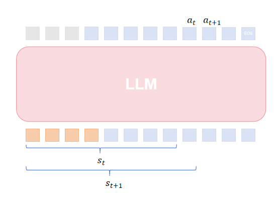
9. RL for Large Language Models (LLMs)

9.1 Modeling in RLHF (Reinforcement Learning from Human Feedback)

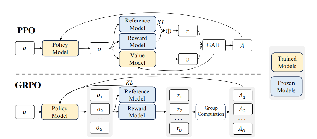
9.2 PPO in RLHF

Original formulation:

\[\operatorname{argmax}_{\boldsymbol{{\theta}^{\prime}}}\mathbf{E}_{s\sim v_{\boldsymbol{\theta}}}\mathbf{E}_{a\sim\pi_{\boldsymbol{\theta}}(\cdot|s)}\left[\min\left(\frac{\pi_{\boldsymbol{{\theta}^{\prime}}}(a|s)}{\pi_{\boldsymbol{\theta}}(a|s)}A_{\pi_{\boldsymbol{\theta}}}^{GAE}(s,a),clip\left(\frac{\pi_{\boldsymbol{{\theta}^{\prime}}}(a|s)}{\pi_{\boldsymbol{\theta}}(a|s)},1-\epsilon,1+\epsilon\right)A_{\pi_{\boldsymbol{\theta}}}^{GAE}(s,a)\right)\right] \]

In RLHF:

\[\mathcal{J}_{PPO}(\theta)=\mathbb{E}\left[q\sim P(Q),o\sim\pi_{\theta_{old}}(O|q)\right]\frac{1}{|o|}\sum_{t=1}^{|o|}\min\left[\frac{\pi_{\theta}(o_{t}|q,o_{<t})}{\pi_{\theta_{old}}(o_{t}|q,o_{<t})}A_{t},\mathrm{clip}\left(\frac{\pi_{\theta}(o_{t}|q,o_{<t})}{\pi_{\theta_{old}}(o_{t}|q,o_{<t})},1-\varepsilon,1+\varepsilon\right)A_{t}\right] \]

\[r_t=r_\varphi(q,o_\leqslant t)-\beta\ln\frac{\pi_\theta(o_t|q,o_{<t})}{\pi_{\theta_{old}}(o_t|q,o_{<t})} \]

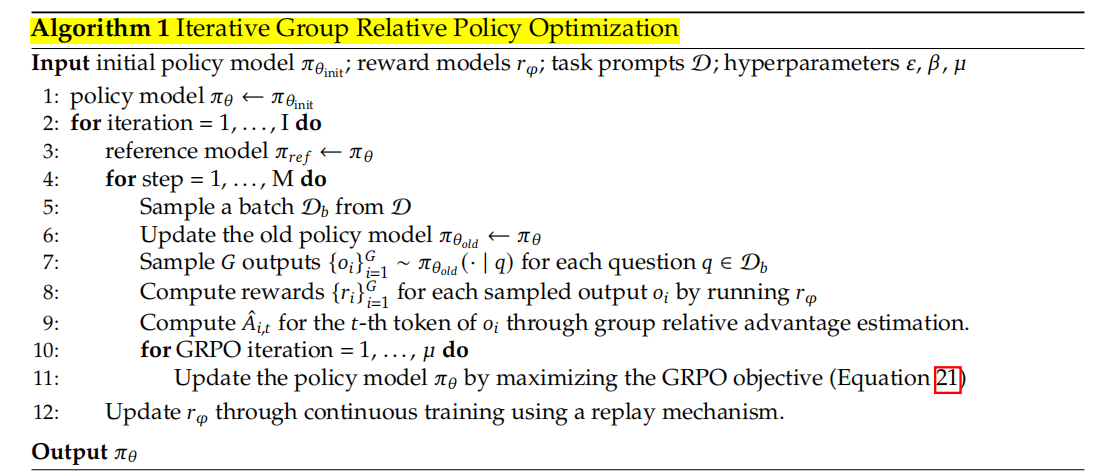
9.3 Group Relative Policy Optimization (GRPO)

\[\mathcal{J}_{\text{GRPO}}(\theta) = \mathbb{E}\left[q \sim P(Q), \{o_i\}_{i=1}^G \sim \pi_{\theta_{\text{old}}}(O|q)\right] \]

\[\left[ \frac{1}{G} \sum_{i=1}^G \frac{1}{|o_i|} \sum_{t=1}^{|o_i|} \left( \min\left( \frac{\pi_\theta(o_{i,t}|q, o_{i,<t})}{\pi_{\theta_{\text{old}}}(o_{i,t}|q, o_{i,<t})} \hat{A}_{i,t}, \text{clip}\left(\frac{\pi_\theta(o_{i,t}|q, o_{i,<t})}{\pi_{\theta_{\text{old}}}(o_{i,t}|q, o_{i,<t})}, 1-\epsilon, 1+\epsilon \right) \hat{A}_{i,t} \right) - \beta \mathbb{D}_{\text{KL}}\left[\pi_\theta \| \pi_{\text{ref}}\right] \right) \right] \]

Normalized advantage function:

\[\hat{A}_{i,t} = \tilde{r}_i = \frac{r_i - \text{mean}(\mathbf{r})}{\text{std}(\mathbf{r})} \]

KL divergence defined as:

\[\mathbb{D}_{\text{KL}}\left[\pi_\theta \| \pi_{\text{ref}}\right] = \frac{\pi_{\text{ref}}(o_{i,t}|q, o_{i,<t})}{\pi_\theta(o_{i,t}|q, o_{i,<t})} - \log \frac{\pi_{\text{ref}}(o_{i,t}|q, o_{i,<t})}{\pi_\theta(o_{i,t}|q, o_{i,<t})} - 1 \]

Reference

https://github.com/MathFoundationRL/Book-Mathematical-Foundation-of-Reinforcement-Learning
https://blog.csdn.net/v_JULY_v/article/details/128965854