TensorFlow实现时间序列预测

　　常常会碰到各种各样时间序列预测问题，如商场人流量的预测、商品价格的预测、股价的预测，等等。TensorFlow新引入了一个TensorFlow Time Series库（以下简称为TFTS），它可以帮助在TensorFlow中快速搭建高性能的时间序列预测系统，并提供包括AR、LSTM在内的多个模型。

时间序列问题

　　一般而言，时间序列数据抽象为两部分：观察的时间点和观察的值（以商品价格为例，某年一月的价格为120元，二月的价格为130元，三月的价格为135元，四月的价格为132元。那么观察的时间点可以看作是1,2,3,4，而在各时间点上观察到的数据的值为120,130,135,132）。观察的时间点可以不连续，比如二月的数据有缺失，那么实际的观察时间点为1,3,4，对应的数据为120,135,132。所谓时间序列预测，是指预测某些未来的时间点上（如5,6）数据的值应该是多少。

　　TFTS库按照时间点+观察值的方式对时间序列问题进行抽象包装。观察的时间点用“times”表示，对应的值用“values”表示。在训练模型时，输入数据需要同时具有times和values两个字段；在预测时，需要给定一些初始的数值，以及需要预测的时间点times。

读入时间序列数据

　　在训练模型之前，需要将时间序列数据读入成Tensor的形式。TFTS库中提供了两个方便的读取器

• NumpyReader：用于从Numpy数组中读入数据
• CSVReader：用于从CSV文件中读入数据

从Numpy数组中读取时间序列

　　导入需要的包及函数

import numpy as np
import matplotlib

matplotlib.use('agg')
import matplotlib.pyplot as plt
import tensorflow as tf
from tensorflow.contrib.timeseries.python.timeseries import NumpyReader

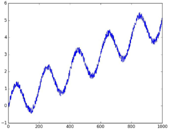
　　接着，利用np.sin生成一个实验用的时间序列数据。该时间序列数据实际上是在正弦曲线上加入了上升的趋势和一些随机的噪声：

x = np.array(range(1000))
noise = np.random.uniform(-0.2, 0.2, 1000)
y = np.sin(np.pi * x / 100) + x / 200. + noise
plt.plot(x, y)
plt.savefig('timeseries_y.jpg')

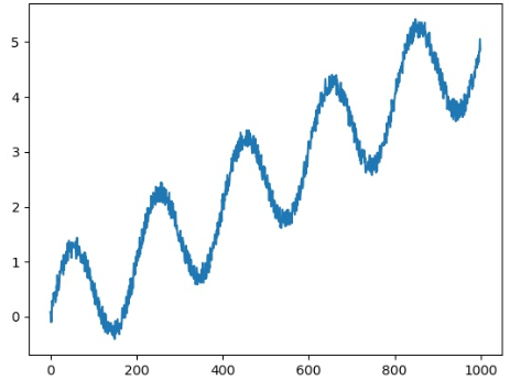
横坐标对应变量“x”，纵坐标对应变量“y”，它们分别对应之前提到过的“观察的时间点”和“观察到的值”。TFTS读入x和y的方式非常简单，请看下面的代码：

data = {
    tf.contrib.timeseries.TrainEvalFeatures.TIMES: x,
    tf.contrib.timeseries.TrainEvalFeatures.VALUES: y,
}

reader = NumpyReader(data)

　　首先把x和y变成Python中的字典（变量data）。上面的定义直接写成“data={‘times':x, ‘values':y}”也是可以的。写成比较复杂的形式是为了和源码中的写法保持一致。

　　得到的reader有一个read_full()方法，它的返回值是时间序列对应的Tensor，可以用下面的代码进行试验：

with tf.Session() as sess:
    full_data = reader.read_full()
    # 调用read_full方法会生成读取队列
    # 要用tf.train.start_queue_runners启动队列才能正常进行读取
    coord = tf.train.Coordinator()
    threads = tf.train.start_queue_runners(sess=sess, coord=coord)
    print(sess.run(full_data))
    coord.request_stop()

　　在训练时，通常不会使用整个数据集进行训练，而是采用batch的形式。从reader出发，建立batch数据的方法也很简单：

train_input_fn = tf.contrib.timeseries.RandomWindowInputFn(
    reader, batch_size=2, window_size=10)

　　tf.contrib.timeseries.RandomWindowInputFn会在reader的所有数据中，随机选取窗口长度为window_size的序列，并包装成batch_size大小的batch数据。换句话说，一个batch内共有batch_size个序列，每个序列的长度为window_size。

　　以batch_size=2, window_size=10为例，可以打印出一个batch的数据：

with tf.Session() as sess:
    batch_data = train_input_fn.create_batch()
    coord = tf.train.Coordinator()
    threads = tf.train.start_queue_runners(sess=sess, coord=coord)
    one_batch = sess.run(batch_data[0])
    coord.request_stop()

print('one_batch_data:', one_batch)
# one_batch_data: {'times': array([[11, 12, 13, 14, 15, 16, 17, 18, 19, 20],
#        [21, 22, 23, 24, 25, 26, 27, 28, 29, 30]]), 'values': array([[[0.33901882],
#         [0.29966548],
#         [0.64006627],
#         [0.35204604],
#         [0.66049626],
#         [0.57470108],
#         [0.68309054],
#         [0.46613038],
#         [0.60309193],
#         [0.84166497]],
# 
#        [[0.77312242],
#         [0.82185951],
#         [0.71022706],
#         [0.63987861],
#         [0.7011966 ],
#         [0.84051192],
#         [1.05796465],
#         [0.92981324],
#         [1.0542786 ],
#         [0.89828743]]])}

　　原先的数据长度为1000的时间序列（x=np.array(range(1000))），使用tf.contrib.timeseries.RandomWindowInputFn，并指定window_size=10, batch_size=2的功能是在这长度为1000的时间序列中，随机选取长度为10的序列，并在每个batch里包含两个这样的序列。这也可以从打印出的数据中看出来。

　　使用tf.contrib.timeseries.RandomWindowInputFn返回的train_input_fn可以进行训练了。这是在TFTS中读入Numpy数组时间序列的基本方式。下面介绍如何读入CSV格式的数据。

从CSV文件中读取时间序列

　　有时，时间序列数据是存在CSV文件中的。当然可以将其先读入为Numpy数组，再使用之前的方法处理。更方便的做法是使用tf.contrib.timeseries.CSVReader读入。数据文件period_trend.csv

　　假设CSV文件的时间序列数据的形式为： 

1,-0.6656603714
2,-0.1164380359
3,0.7398626488
4,0.7368633029
5,0.2289480898
...

　　CSV文件的第一列为时间点，第二列为该时间点上观察到的值。将其读入的方法为：

import tensorflow as tf

csv_file_name = './period_trend.csv'
reader = tf.contrib.timeseries.CSVReader(csv_file_name)

　　实际读入的代码只有一行，直接使用函数tf.contrib.timeseries.CSVReader得到了reader。将reader中所有数据打印出来的方法和之前是一样的：

with tf.Session() as sess:
    data = reader.read_full()
    coord = tf.train.Coordinator()
    threads = tf.train.start_queue_runners(sess=sess, coord=coord)
    print(sess.run(data))
    coord.request_stop()

　　从reader出发，建立batch数据的train_input_fn的方法也完全相同：

train_input_fn = tf.contrib.timeseries.RandomWindowInputFn(reader, batch_size=4, window_size=16)

　　最后，可以打印出两个batch的数据进行测试：

with tf.Session() as sess:
    data = train_input_fn.create_batch()
    coord = tf.train.Coordinator()
    threads = tf.train.start_queue_runners(sess=sess, coord=coord)
    batch1 = sess.run(data[0])
    batch2 = sess.run(data[0])
    coord.request_stop()

print('batch1:', batch1)
print('batch2:', batch2)

　　以上是TFTS库中数据的读取方式。总的来说，从Numpy数组或者CSV文件出发构造一个reader，再利用reader生成batch数据。最后得到的Tensor为train_input_fn，这个train_input_fn会被当作训练时的输入。

使用AR模型预测时间序列

AR模型的训练

　　自回归模型（Autoregressive model，简称为AR模型）是统计学上处理时间序列模型的基本方法之一。TFTS中已经实现了一个自回归模型，我们只需要对其进行调用即可使用。

我们先定义出一个train_input_fn

x = np.array(range(1000))
noise = np.random.uniform(-0.2, 0.2, 1000)
y = np.sin(np.pi * x / 100) + x / 200. + noise
plt.plot(x, y)
plt.savefig('timeseries_y.jpg')

data = {
    tf.contrib.timeseries.TrainEvalFeatures.TIMES: x,
    tf.contrib.timeseries.TrainEvalFeatures.VALUES: y,
}

reader = NumpyReader(data)

train_input_fn = tf.contrib.timeseries.RandomWindowInputFn(
    reader, batch_size=16, window_size=40)

使用的时间序列数据如图所示。

　　定义AR模型：

ar = tf.contrib.timeseries.ARRegressor(
    periodicities=200, input_window_size=30, output_window_size=10,
    num_features=1,
    loss=tf.contrib.timeseries.ARModel.NORMAL_LIKELIHOOD_LOSS)

参数：

• periodicities：序列的规律性周期。在定义数据时使用的语句是“y=np.sin(np.pi * x /100)+x /200.+noise”，因此周期为200
• input_window_size：模型每次输入的值
• output_window_size：模型每次输出的值
• num_features：表示在一个时间点上观察到的数的维度。这里每一步都是一个单独的值，所以num_features=1
• loss：指定采取哪一种损失，NORMAL_LIKELIHOOD_LOSS 或 SQUARED_LOSS
• model_dir：模型训练好后保存的地址，如果不指定的话，会随机分配一个临时地址

　　input_window_size和output_window_size加起来必须等于train_input_fn中总的window_size。总的window_size为40, input_window_size为30,output_window_size为10；也是说，一个batch内每个序列的长度为40，其中前30个数被当作模型的输入值，后面10个数为这些输入对应的目标输出值。

　　使用变量ar的train方法可以直接进行训练：

ar.train(input_fn=train_input_fn, steps=6000)

AR模型的验证和预测

　　TFTS中验证（evaluation）的含义是：使用训练好的模型在原先的训练集上进行计算，由此可以观察到模型的拟合效果，对应的程序段是：

evaluation_input_fn = tf.contrib.timeseries.WholeDatasetInputFn(reader)
# keys of evaluation: ['covariance', 'loss', 'mean', 'observed', 'start_tuple', 'times', 'global_step']
evaluation = ar.evaluate(input_fn=evaluation_input_fn, steps=1)

　　如果想要明白这里的逻辑，首先要理解之前定义的AR模型：它每次都接收一个长度为30的输入观测序列，并输出长度为10的预测序列。整个训练集是一个长度为1000的序列，前30个数首先被当作“初始观测序列”输入到模型中，由此可以计算出下面10步的预测值。接着又会取30个数进行预测，这30个数中有10个数是前一步的预测值，新得到的预测值又会变成下一步的输入，依此类推。

　　最终得到970个预测值（970=1000-30，因为前30个数是没办法进行预测的）。970个预测值被记录在evaluation[‘mean']中。evaluation还有其他几个键值，如evaluation[‘times']表示evaluation[‘mean']对应的时间点，evaluation[‘loss']表示总的损失等等。

　　evaluation[‘start_tuple']会被用于之后的预测中，它相当于最后30步的输出值和对应的时间点。以此为起点，可以对1000步以后的值进行预测，对应的代码为：

(predictions,) = tuple(ar.predict(
    input_fn=tf.contrib.timeseries.predict_continuation_input_fn(
        evaluation, steps=250)))

　　这里的代码在1000步之后又向后预测了250个时间点。对应的值保存在predictions[‘mean']中。可以把观测到的值、模型拟合的值、预测值用下面的代码画出来：

plt.figure(figsize=(15, 5))
plt.plot(data['times'].reshape(-1), data['values'].reshape(-1), label='origin')
plt.plot(evaluation['times'].reshape(-1), evaluation['mean'].reshape(-1), label='evaluation')
plt.plot(predictions['times'].reshape(-1), predictions['mean'].reshape(-1), label='prediction')
plt.xlabel('time_step')
plt.ylabel('values')
plt.legend(loc=4)
plt.savefig('predict_result.jpg')

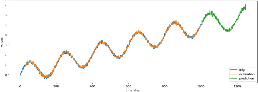
　　前1000步模型原始观测值的曲线和模型拟合值非常接近，说明模型拟合得已经比较好了，1000步之后的预测也合情合理。

# coding: utf-8
from __future__ import print_function
import numpy as np
import matplotlib
matplotlib.use('agg')
import matplotlib.pyplot as plt
import tensorflow as tf
from tensorflow.contrib.timeseries.python.timeseries import  NumpyReader


def main(_):
    x = np.array(range(1000))
    noise = np.random.uniform(-0.2, 0.2, 1000)
    y = np.sin(np.pi * x / 100) + x / 200. + noise
    plt.plot(x, y)
    plt.savefig('timeseries_y.jpg')

    data = {
        tf.contrib.timeseries.TrainEvalFeatures.TIMES: x,
        tf.contrib.timeseries.TrainEvalFeatures.VALUES: y,
    }

    reader = NumpyReader(data)

    train_input_fn = tf.contrib.timeseries.RandomWindowInputFn(
        reader, batch_size=16, window_size=40)

    ar = tf.contrib.timeseries.ARRegressor(
        periodicities=200, input_window_size=30, output_window_size=10,
        num_features=1,
        loss=tf.contrib.timeseries.ARModel.NORMAL_LIKELIHOOD_LOSS)

    ar.train(input_fn=train_input_fn, steps=6000)

    evaluation_input_fn = tf.contrib.timeseries.WholeDatasetInputFn(reader)
    # keys of evaluation: ['covariance', 'loss', 'mean', 'observed', 'start_tuple', 'times', 'global_step']
    evaluation = ar.evaluate(input_fn=evaluation_input_fn, steps=1)

    (predictions,) = tuple(ar.predict(
        input_fn=tf.contrib.timeseries.predict_continuation_input_fn(
            evaluation, steps=250)))

    plt.figure(figsize=(15, 5))
    plt.plot(data['times'].reshape(-1), data['values'].reshape(-1), label='origin')
    plt.plot(evaluation['times'].reshape(-1), evaluation['mean'].reshape(-1), label='evaluation')
    plt.plot(predictions['times'].reshape(-1), predictions['mean'].reshape(-1), label='prediction')
    plt.xlabel('time_step')
    plt.ylabel('values')
    plt.legend(loc=4)
    plt.savefig('predict_result.jpg')


if __name__ == '__main__':
    tf.logging.set_verbosity(tf.logging.INFO)
    tf.app.run()

使用LSTM模型预测时间序列

　　为了使用LSTM模型，需要先使用TFTS库对其进行定义。

单变量时间序列预测

　　同样，用函数加噪声的方法模拟生成时间序列数据：

x = np.array(range(1000))
noise = np.random.uniform(-0.2, 0.2, 1000)
y = np.sin(np.pi * x / 50) + np.cos(np.pi * x / 50) + np.sin(np.pi * x / 25) + noise

data = {
    tf.contrib.timeseries.TrainEvalFeatures.TIMES: x,
    tf.contrib.timeseries.TrainEvalFeatures.VALUES: y,
}

reader = NumpyReader(data)

train_input_fn = tf.contrib.timeseries.RandomWindowInputFn(
    reader, batch_size=4, window_size=100)

　　得到y和x后，使用NumpyReader读入为Tensor形式，接着用tf.contrib.timeseries.RandomWindowInputFn将其变为batch训练数据。一个batch中有4个随机选取的序列，每个序列的长度为100。

　　接下来定义一个LSTM模型：

estimator = ts_estimators.TimeSeriesRegressor(
        model=_LSTMModel(num_features=1, num_units=128),
        optimizer=tf.train.AdamOptimizer(0.001))

　　num_features=1表示单变量时间序列，即每个时间点上观察到的量只是一个单独的数值，num_units=128表示使用隐层为128大小的LSTM模型。

　　训练、验证和预测的方法都和之前类似。在训练时，在已有的1000步的观察量的基础上向后预测200步：

estimator.train(input_fn=train_input_fn, steps=2000)　　　　# 训练模型
evaluation_input_fn = tf.contrib.timeseries.WholeDatasetInputFn(reader)　　# 测试数据
evaluation = estimator.evaluate(input_fn=evaluation_input_fn, steps=1)　　# 得到评估后的数据
# 评估后预测200步数据
(predictions,) = tuple(estimator.predict(
    input_fn=tf.contrib.timeseries.predict_continuation_input_fn(
        evaluation, steps=200)))

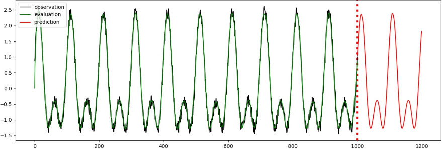
将验证、预测的结果取出并画成示意图，画出的图像会保存成“predict_result.jpg”文件：

observed_times = evaluation["times"][0]
observed = evaluation["observed"][0, :, :]
evaluated_times = evaluation["times"][0]
evaluated = evaluation["mean"][0]
predicted_times = predictions['times']
predicted = predictions["mean"]

plt.figure(figsize=(15, 5))
plt.axvline(999, linestyle="dotted", linewidth=4, color='r')
observed_lines = plt.plot(observed_times, observed, label="observation", color="k")
evaluated_lines = plt.plot(evaluated_times, evaluated, label="evaluation", color="g")
predicted_lines = plt.plot(predicted_times, predicted, label="prediction", color="r")
plt.legend(handles=[observed_lines[0], evaluated_lines[0], predicted_lines[0]],
           loc="upper left")
plt.savefig('predict_result.jpg')

预测效果如图15-4所示，横坐标为时间轴，前1000步是训练数据，1000~1200步是模型预测的值。

import numpy as np
import tensorflow as tf

from tensorflow.contrib.timeseries.python.timeseries import estimators as ts_estimators
from tensorflow.contrib.timeseries.python.timeseries import model as ts_model
from tensorflow.contrib.timeseries.python.timeseries import NumpyReader

import matplotlib

matplotlib.use("agg")
import matplotlib.pyplot as plt


class _LSTMModel(ts_model.SequentialTimeSeriesModel):
    """A time series model-building example using an RNNCell."""

    def __init__(self, num_units, num_features, dtype=tf.float32):
        """Initialize/configure the model object.
        Note that we do not start graph building here. Rather, this object is a
        configurable factory for TensorFlow graphs which are run by an Estimator.
        Args:
          num_units: The number of units in the model's LSTMCell.
          num_features: The dimensionality of the time series (features per
            timestep).
          dtype: The floating point data type to use.
        """
        super(_LSTMModel, self).__init__(
            # Pre-register the metrics we'll be outputting (just a mean here).
            train_output_names=["mean"],
            predict_output_names=["mean"],
            num_features=num_features,
            dtype=dtype)
        self._num_units = num_units
        # Filled in by initialize_graph()
        self._lstm_cell = None
        self._lstm_cell_run = None
        self._predict_from_lstm_output = None

    def initialize_graph(self, input_statistics):
        """Save templates for components, which can then be used repeatedly.
        This method is called every time a new graph is created. It's safe to start
        adding ops to the current default graph here, but the graph should be
        constructed from scratch.
        Args:
          input_statistics: A math_utils.InputStatistics object.
        """
        super(_LSTMModel, self).initialize_graph(input_statistics=input_statistics)
        self._lstm_cell = tf.nn.rnn_cell.LSTMCell(num_units=self._num_units)
        # Create templates so we don't have to worry about variable reuse.
        self._lstm_cell_run = tf.make_template(
            name_="lstm_cell",
            func_=self._lstm_cell,
            create_scope_now_=True)
        # Transforms LSTM output into mean predictions.
        self._predict_from_lstm_output = tf.make_template(
            name_="predict_from_lstm_output",
            func_=lambda inputs: tf.layers.dense(inputs=inputs, units=self.num_features),
            create_scope_now_=True)

    def get_start_state(self):
        """Return initial state for the time series model."""
        return (
            # Keeps track of the time associated with this state for error checking.
            tf.zeros([], dtype=tf.int64),
            # The previous observation or prediction.
            tf.zeros([self.num_features], dtype=self.dtype),
            # The state of the RNNCell (batch dimension removed since this parent
            # class will broadcast).
            [tf.squeeze(state_element, axis=0)
             for state_element
             in self._lstm_cell.zero_state(batch_size=1, dtype=self.dtype)])

    def _transform(self, data):
        """Normalize data based on input statistics to encourage stable training."""
        mean, variance = self._input_statistics.overall_feature_moments
        return (data - mean) / variance

    def _de_transform(self, data):
        """Transform data back to the input scale."""
        mean, variance = self._input_statistics.overall_feature_moments
        return data * variance + mean

    def _filtering_step(self, current_times, current_values, state, predictions):
        """Update model state based on observations.
        Note that we don't do much here aside from computing a loss. In this case
        it's easier to update the RNN state in _prediction_step, since that covers
        running the RNN both on observations (from this method) and our own
        predictions. This distinction can be important for probabilistic models,
        where repeatedly predicting without filtering should lead to low-confidence
        predictions.
        Args:
          current_times: A [batch size] integer Tensor.
          current_values: A [batch size, self.num_features] floating point Tensor
            with new observations.
          state: The model's state tuple.
          predictions: The output of the previous `_prediction_step`.
        Returns:
          A tuple of new state and a predictions dictionary updated to include a
          loss (note that we could also return other measures of goodness of fit,
          although only "loss" will be optimized).
        """
        state_from_time, prediction, lstm_state = state
        with tf.control_dependencies(
                [tf.assert_equal(current_times, state_from_time)]):
            transformed_values = self._transform(current_values)
            # Use mean squared error across features for the loss.
            predictions["loss"] = tf.reduce_mean(
                (prediction - transformed_values) ** 2, axis=-1)
            # Keep track of the new observation in model state. It won't be run
            # through the LSTM until the next _imputation_step.
            new_state_tuple = (current_times, transformed_values, lstm_state)
        return (new_state_tuple, predictions)

    def _prediction_step(self, current_times, state):
        """Advance the RNN state using a previous observation or prediction."""
        _, previous_observation_or_prediction, lstm_state = state
        lstm_output, new_lstm_state = self._lstm_cell_run(
            inputs=previous_observation_or_prediction, state=lstm_state)
        next_prediction = self._predict_from_lstm_output(lstm_output)
        new_state_tuple = (current_times, next_prediction, new_lstm_state)
        return new_state_tuple, {"mean": self._de_transform(next_prediction)}

    def _imputation_step(self, current_times, state):
        """Advance model state across a gap."""
        # Does not do anything special if we're jumping across a gap. More advanced
        # models, especially probabilistic ones, would want a special case that
        # depends on the gap size.
        return state

    def _exogenous_input_step(
            self, current_times, current_exogenous_regressors, state):
        """Update model state based on exogenous regressors."""
        raise NotImplementedError(
            "Exogenous inputs are not implemented for this example.")


if __name__ == '__main__':
    tf.logging.set_verbosity(tf.logging.INFO)
    x = np.array(range(1000))
    noise = np.random.uniform(-0.2, 0.2, 1000)
    y = np.sin(np.pi * x / 50) + np.cos(np.pi * x / 50) + np.sin(np.pi * x / 25) + noise

    data = {
        tf.contrib.timeseries.TrainEvalFeatures.TIMES: x,
        tf.contrib.timeseries.TrainEvalFeatures.VALUES: y,
    }

    reader = NumpyReader(data)

    train_input_fn = tf.contrib.timeseries.RandomWindowInputFn(
        reader, batch_size=4, window_size=100)

    estimator = ts_estimators.TimeSeriesRegressor(
        model=_LSTMModel(num_features=1, num_units=128),
        optimizer=tf.train.AdamOptimizer(0.001))

    estimator.train(input_fn=train_input_fn, steps=2000)
    evaluation_input_fn = tf.contrib.timeseries.WholeDatasetInputFn(reader)
    evaluation = estimator.evaluate(input_fn=evaluation_input_fn, steps=1)
    # Predict starting after the evaluation
    (predictions,) = tuple(estimator.predict(
        input_fn=tf.contrib.timeseries.predict_continuation_input_fn(
            evaluation, steps=200)))

    observed_times = evaluation["times"][0]
    observed = evaluation["observed"][0, :, :]
    evaluated_times = evaluation["times"][0]
    evaluated = evaluation["mean"][0]
    predicted_times = predictions['times']
    predicted = predictions["mean"]

    plt.figure(figsize=(15, 5))
    plt.axvline(999, linestyle="dotted", linewidth=4, color='r')
    observed_lines = plt.plot(observed_times, observed, label="observation", color="k")
    evaluated_lines = plt.plot(evaluated_times, evaluated, label="evaluation", color="g")
    predicted_lines = plt.plot(predicted_times, predicted, label="prediction", color="r")
    plt.legend(handles=[observed_lines[0], evaluated_lines[0], predicted_lines[0]],
               loc="upper left")
    plt.savefig('predict_result.jpg')

多变量时间序列预测

　　所谓多变量时间序列，是指在每个时间点上的观测量有多个值。在multivariate_periods.csv文件中，保存了一个多变量时间序列的数据：

0    0.926906299771    1.99107237682    2.56546245685    3.07914768197    4.04839057867
1    0.108010001864    1.41645361423    2.1686839775    2.94963962176    4.1263503303
2    -0.800567600028    1.0172132907    1.96434754116    2.99885333086    4.04300485864
3    0.0607042871898    0.719540073421    1.9765012584    2.89265588817    4.0951014426
...
99    0.987764008058    1.85581989607    2.84685706149    2.94760204892    6.0212151724

　　这个CSV文件的第一列是观察时间点，除此之外，每一行还有5个数，表示在这个时间点上观察到的数据。换句话说，时间序列上每一步都是一个5维的向量。

　　使用TFTS读入该CSV文件的方法为：

csv_file_name = path.join("./data/multivariate_periods.csv")
reader = tf.contrib.timeseries.CSVReader(
    csv_file_name,
    column_names=((tf.contrib.timeseries.TrainEvalFeatures.TIMES,)
                  + (tf.contrib.timeseries.TrainEvalFeatures.VALUES,) * 5))
train_input_fn = tf.contrib.timeseries.RandomWindowInputFn(
    reader, batch_size=4, window_size=32)

　　与之前的读入相比，唯一的区别是column_names参数。它告诉TFTS在CSV文件中，哪些列表示时间，哪些列表示观测量。

　　接下来定义LSTM模型：

estimator = ts_estimators.TimeSeriesRegressor(
    model=_LSTMModel(num_features=5, num_units=128),
    optimizer=tf.train.AdamOptimizer(0.001))

　　区别在于使用num_features=5而不是1，原因在于每个时间点上的观测量是一个5维向量。

　　训练、验证、预测及画图的代码与之前比较类似，最后的运行结果图所示

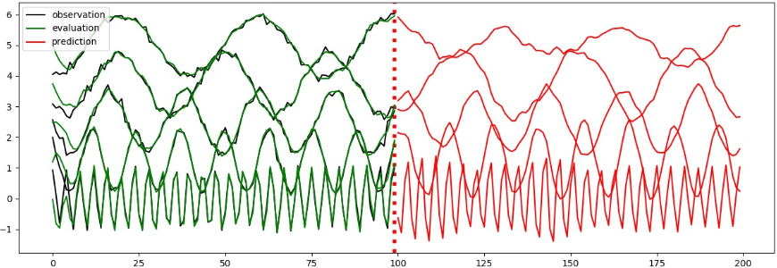
使用LSTM预测多变量时间序列

　　前100步是训练数据，一条线代表观测量在一个维度上的取值。100步之后为预测值。

from os import path
import tensorflow as tf

from tensorflow.contrib.timeseries.python.timeseries import estimators as ts_estimators
from tensorflow.contrib.timeseries.python.timeseries import model as ts_model
import matplotlib

matplotlib.use("agg")
import matplotlib.pyplot as plt


class _LSTMModel(ts_model.SequentialTimeSeriesModel):
    """A time series model-building example using an RNNCell."""

    def __init__(self, num_units, num_features, dtype=tf.float32):
        """Initialize/configure the model object.
        Note that we do not start graph building here. Rather, this object is a
        configurable factory for TensorFlow graphs which are run by an Estimator.
        Args:
          num_units: The number of units in the model's LSTMCell.
          num_features: The dimensionality of the time series (features per
            timestep).
          dtype: The floating point data type to use.
        """
        super(_LSTMModel, self).__init__(
            # Pre-register the metrics we'll be outputting (just a mean here).
            train_output_names=["mean"],
            predict_output_names=["mean"],
            num_features=num_features,
            dtype=dtype)
        self._num_units = num_units
        # Filled in by initialize_graph()
        self._lstm_cell = None
        self._lstm_cell_run = None
        self._predict_from_lstm_output = None

    def initialize_graph(self, input_statistics):
        """Save templates for components, which can then be used repeatedly.
        This method is called every time a new graph is created. It's safe to start
        adding ops to the current default graph here, but the graph should be
        constructed from scratch.
        Args:
          input_statistics: A math_utils.InputStatistics object.
        """
        super(_LSTMModel, self).initialize_graph(input_statistics=input_statistics)
        self._lstm_cell = tf.nn.rnn_cell.LSTMCell(num_units=self._num_units)
        # Create templates so we don't have to worry about variable reuse.
        self._lstm_cell_run = tf.make_template(
            name_="lstm_cell",
            func_=self._lstm_cell,
            create_scope_now_=True)
        # Transforms LSTM output into mean predictions.
        self._predict_from_lstm_output = tf.make_template(
            name_="predict_from_lstm_output",
            func_=lambda inputs: tf.layers.dense(inputs=inputs, units=self.num_features),
            create_scope_now_=True)

    def get_start_state(self):
        """Return initial state for the time series model."""
        return (
            # Keeps track of the time associated with this state for error checking.
            tf.zeros([], dtype=tf.int64),
            # The previous observation or prediction.
            tf.zeros([self.num_features], dtype=self.dtype),
            # The state of the RNNCell (batch dimension removed since this parent
            # class will broadcast).
            [tf.squeeze(state_element, axis=0)
             for state_element
             in self._lstm_cell.zero_state(batch_size=1, dtype=self.dtype)])

    def _transform(self, data):
        """Normalize data based on input statistics to encourage stable training."""
        mean, variance = self._input_statistics.overall_feature_moments
        return (data - mean) / variance

    def _de_transform(self, data):
        """Transform data back to the input scale."""
        mean, variance = self._input_statistics.overall_feature_moments
        return data * variance + mean

    def _filtering_step(self, current_times, current_values, state, predictions):
        """Update model state based on observations.
        Note that we don't do much here aside from computing a loss. In this case
        it's easier to update the RNN state in _prediction_step, since that covers
        running the RNN both on observations (from this method) and our own
        predictions. This distinction can be important for probabilistic models,
        where repeatedly predicting without filtering should lead to low-confidence
        predictions.
        Args:
          current_times: A [batch size] integer Tensor.
          current_values: A [batch size, self.num_features] floating point Tensor
            with new observations.
          state: The model's state tuple.
          predictions: The output of the previous `_prediction_step`.
        Returns:
          A tuple of new state and a predictions dictionary updated to include a
          loss (note that we could also return other measures of goodness of fit,
          although only "loss" will be optimized).
        """
        state_from_time, prediction, lstm_state = state
        with tf.control_dependencies(
                [tf.assert_equal(current_times, state_from_time)]):
            transformed_values = self._transform(current_values)
            # Use mean squared error across features for the loss.
            predictions["loss"] = tf.reduce_mean(
                (prediction - transformed_values) ** 2, axis=-1)
            # Keep track of the new observation in model state. It won't be run
            # through the LSTM until the next _imputation_step.
            new_state_tuple = (current_times, transformed_values, lstm_state)
        return (new_state_tuple, predictions)

    def _prediction_step(self, current_times, state):
        """Advance the RNN state using a previous observation or prediction."""
        _, previous_observation_or_prediction, lstm_state = state
        lstm_output, new_lstm_state = self._lstm_cell_run(
            inputs=previous_observation_or_prediction, state=lstm_state)
        next_prediction = self._predict_from_lstm_output(lstm_output)
        new_state_tuple = (current_times, next_prediction, new_lstm_state)
        return new_state_tuple, {"mean": self._de_transform(next_prediction)}

    def _imputation_step(self, current_times, state):
        """Advance model state across a gap."""
        # Does not do anything special if we're jumping across a gap. More advanced
        # models, especially probabilistic ones, would want a special case that
        # depends on the gap size.
        return state

    def _exogenous_input_step(
            self, current_times, current_exogenous_regressors, state):
        """Update model state based on exogenous regressors."""
        raise NotImplementedError(
            "Exogenous inputs are not implemented for this example.")


if __name__ == '__main__':
    tf.logging.set_verbosity(tf.logging.INFO)
    csv_file_name = path.join("./data/multivariate_periods.csv")
    reader = tf.contrib.timeseries.CSVReader(
        csv_file_name,
        column_names=((tf.contrib.timeseries.TrainEvalFeatures.TIMES,)
                      + (tf.contrib.timeseries.TrainEvalFeatures.VALUES,) * 5))
    train_input_fn = tf.contrib.timeseries.RandomWindowInputFn(
        reader, batch_size=4, window_size=32)

    estimator = ts_estimators.TimeSeriesRegressor(
        model=_LSTMModel(num_features=5, num_units=128),
        optimizer=tf.train.AdamOptimizer(0.001))

    estimator.train(input_fn=train_input_fn, steps=200)
    evaluation_input_fn = tf.contrib.timeseries.WholeDatasetInputFn(reader)
    evaluation = estimator.evaluate(input_fn=evaluation_input_fn, steps=1)
    # Predict starting after the evaluation
    (predictions,) = tuple(estimator.predict(
        input_fn=tf.contrib.timeseries.predict_continuation_input_fn(
            evaluation, steps=100)))

    observed_times = evaluation["times"][0]
    observed = evaluation["observed"][0, :, :]
    evaluated_times = evaluation["times"][0]
    evaluated = evaluation["mean"][0]
    predicted_times = predictions['times']
    predicted = predictions["mean"]

    plt.figure(figsize=(15, 5))
    plt.axvline(99, linestyle="dotted", linewidth=4, color='r')
    observed_lines = plt.plot(observed_times, observed, label="observation", color="k")
    evaluated_lines = plt.plot(evaluated_times, evaluated, label="evaluation", color="g")
    predicted_lines = plt.plot(predicted_times, predicted, label="prediction", color="r")
    plt.legend(handles=[observed_lines[0], evaluated_lines[0], predicted_lines[0]],
               loc="upper left")
    plt.savefig('predict_result.jpg')