分类问题--二分类Logistic回归

参考《深度学习入门之PyTorch》--廖星宇
书籍配套GitHub链接
https://github.com/L1aoXingyu/code-of-learn-deep-learning-with-pytorch/blob/master/chapter3_NN/logistic-regression/logistic-regression.ipynb
GitHub内容适应Pytorch版本0.3.0
博客中将程序修改为适应Pytorch 1.0

sigmoid函数图像

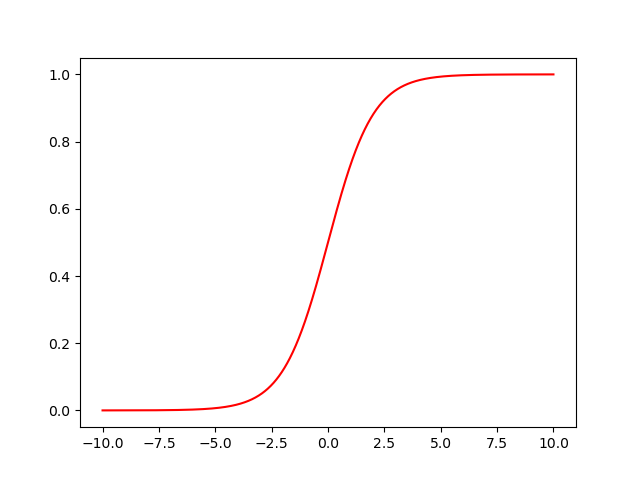
# 定义 sigmoid 函数
def sigmoid(x):
    return 1 / (1 + np.exp(-x))


# 画出 sigmoid 的图像
plot_x = np.arange(-10, 10.01, 0.01)
plot_y = sigmoid(plot_x)

plt.plot(plot_x, plot_y, 'r')
plt.show()

从 data.txt 读入数据
data内容

34.62365962451697,78.0246928153624,0
30.28671076822607,43.89499752400101,0
35.84740876993872,72.90219802708364,0
60.18259938620976,86.30855209546826,1
79.0327360507101,75.3443764369103,1
45.08327747668339,56.3163717815305,0
61.10666453684766,96.51142588489624,1
75.02474556738889,46.55401354116538,1
76.09878670226257,87.42056971926803,1
84.43281996120035,43.53339331072109,1
95.86155507093572,38.22527805795094,0
75.01365838958247,30.60326323428011,0
82.30705337399482,76.48196330235604,1
69.36458875970939,97.71869196188608,1
39.53833914367223,76.03681085115882,0
53.9710521485623,89.20735013750205,1
69.07014406283025,52.74046973016765,1
67.94685547711617,46.67857410673128,0
70.66150955499435,92.92713789364831,1
76.97878372747498,47.57596364975532,1
67.37202754570876,42.83843832029179,0
89.67677575072079,65.79936592745237,1
50.534788289883,48.85581152764205,0
34.21206097786789,44.20952859866288,0
77.9240914545704,68.9723599933059,1
62.27101367004632,69.95445795447587,1
80.1901807509566,44.82162893218353,1
93.114388797442,38.80067033713209,0
61.83020602312595,50.25610789244621,0
38.78580379679423,64.99568095539578,0
61.379289447425,72.80788731317097,1
85.40451939411645,57.05198397627122,1
52.10797973193984,63.12762376881715,0
52.04540476831827,69.43286012045222,1
40.23689373545111,71.16774802184875,0
54.63510555424817,52.21388588061123,0
33.91550010906887,98.86943574220611,0
64.17698887494485,80.90806058670817,1
74.78925295941542,41.57341522824434,0
34.1836400264419,75.2377203360134,0
83.90239366249155,56.30804621605327,1
51.54772026906181,46.85629026349976,0
94.44336776917852,65.56892160559052,1
82.36875375713919,40.61825515970618,0
51.04775177128865,45.82270145776001,0
62.22267576120188,52.06099194836679,0
77.19303492601364,70.45820000180959,1
97.77159928000232,86.7278223300282,1
62.07306379667647,96.76882412413983,1
91.56497449807442,88.69629254546599,1
79.94481794066932,74.16311935043758,1
99.2725269292572,60.99903099844988,1
90.54671411399852,43.39060180650027,1
34.52451385320009,60.39634245837173,0
50.2864961189907,49.80453881323059,0
49.58667721632031,59.80895099453265,0
97.64563396007767,68.86157272420604,1
32.57720016809309,95.59854761387875,0
74.24869136721598,69.82457122657193,1
71.79646205863379,78.45356224515052,1
75.3956114656803,85.75993667331619,1
35.28611281526193,47.02051394723416,0
56.25381749711624,39.26147251058019,0
30.05882244669796,49.59297386723685,0
44.66826172480893,66.45008614558913,0
66.56089447242954,41.09209807936973,0
40.45755098375164,97.53518548909936,1
49.07256321908844,51.88321182073966,0
80.27957401466998,92.11606081344084,1
66.74671856944039,60.99139402740988,1
32.72283304060323,43.30717306430063,0
64.0393204150601,78.03168802018232,1
72.34649422579923,96.22759296761404,1
60.45788573918959,73.09499809758037,1
58.84095621726802,75.85844831279042,1
99.82785779692128,72.36925193383885,1
47.26426910848174,88.47586499559782,1
50.45815980285988,75.80985952982456,1
60.45555629271532,42.50840943572217,0
82.22666157785568,42.71987853716458,0
88.9138964166533,69.80378889835472,1
94.83450672430196,45.69430680250754,1
67.31925746917527,66.58935317747915,1
57.23870631569862,59.51428198012956,1
80.36675600171273,90.96014789746954,1
68.46852178591112,85.59430710452014,1
42.0754545384731,78.84478600148043,0
75.47770200533905,90.42453899753964,1
78.63542434898018,96.64742716885644,1
52.34800398794107,60.76950525602592,0
94.09433112516793,77.15910509073893,1
90.44855097096364,87.50879176484702,1
55.48216114069585,35.57070347228866,0
74.49269241843041,84.84513684930135,1
89.84580670720979,45.35828361091658,1
83.48916274498238,48.38028579728175,1
42.2617008099817,87.10385094025457,1
99.31500880510394,68.77540947206617,1
55.34001756003703,64.9319380069486,1
74.77589300092767,89.52981289513276,1

例如：74.77589300092767,89.52981289513276,1
74.77589300092767,89.52981289513276代表横纵坐标，1/0代表两种类型
下图是data内容绘图展示

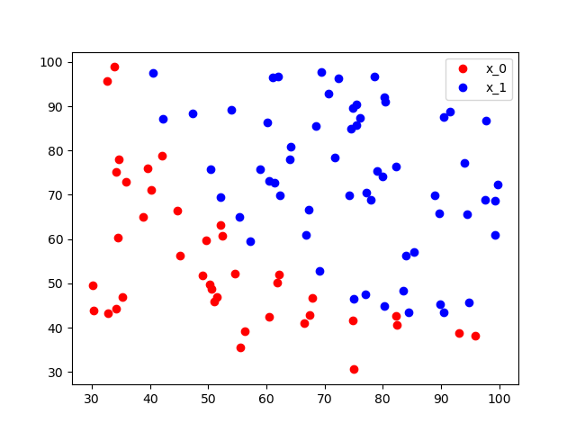
红蓝两类点是线性可分的

import torch
from torch.autograd import Variable
import numpy as np
import matplotlib.pyplot as plt
from torch import nn
import time

# 设定随机种子
torch.manual_seed(2017)

# 从 data.txt 中读入点
with open('./data.txt', 'r') as f:
    data_list = [i.split('\n')[0].split(',') for i in f.readlines()]
    data = [(float(i[0]), float(i[1]), float(i[2])) for i in data_list]

# 坐标归一化到[0 ~1]
x0_max = max([i[0] for i in data])
x1_max = max([i[1] for i in data])
data = [(i[0]/x0_max, i[1]/x1_max, i[2]) for i in data]

# 分类
x0 = list(filter(lambda x: x[-1] == 0.0, data)) # 选择第一类的点
x1 = list(filter(lambda x: x[-1] == 1.0, data)) # 选择第二类的点

plot_x0 = [i[0] for i in x0]
plot_y0 = [i[1] for i in x0]
plot_x1 = [i[0] for i in x1]
plot_y1 = [i[1] for i in x1]

plt.plot(plot_x0, plot_y0, 'ro', label='x_0')
plt.plot(plot_x1, plot_y1, 'bo', label='x_1')
plt.legend(loc='best')
plt.show()

np_data = np.array(data, dtype='float32')  # 转换成 numpy array
x_data = torch.from_numpy(np_data[:, 0:2])  # 转换成 Tensor, 大小是 [100, 2]
y_data = torch.from_numpy(np_data[:, -1]).unsqueeze(1)  # 转换成 Tensor，大小是 [100, 1]
x_data = Variable(x_data)
y_data = Variable(y_data)

# 定义 logistic 回归模型
w = Variable(torch.randn(2, 1), requires_grad=True)
b = Variable(torch.zeros(1), requires_grad=True)


def logistic_regression(x):
    return torch.sigmoid(torch.mm(x, w) + b)


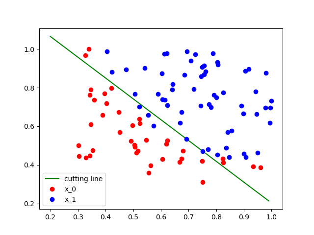
# 画出参数更新之前的结果
w0 = float(w[0].data[0])
w1 = float(w[1].data[0])
b0 = float(b.data[0])

plot_x = np.arange(0.2, 1, 0.01)
plot_y = (-w0 * plot_x - b0) / w1


plt.plot(plot_x, plot_y, 'g', label='cutting line')
plt.plot(plot_x0, plot_y0, 'ro', label='x_0')
plt.plot(plot_x1, plot_y1, 'bo', label='x_1')
plt.legend(loc='best')
plt.show()


# 计算loss
def binary_loss(y_pred, y):
    logits = (y * y_pred.clamp(1e-12).log() + (1 - y) * (1 - y_pred).clamp(1e-12).log()).mean()
    return -logits

y_pred = logistic_regression(x_data)
loss = binary_loss(y_pred, y_data)
print(loss)

# 自动求导并更新参数
loss.backward()
w.data = w.data - 0.1 * w.grad.data
b.data = b.data - 0.1 * b.grad.data

# 算出一次更新之后的loss
y_pred = logistic_regression(x_data)
loss = binary_loss(y_pred, y_data)
print(loss)


# 使用 torch.optim 更新参数

w = nn.Parameter(torch.randn(2, 1))
b = nn.Parameter(torch.zeros(1))

def logistic_regression(x):
    return torch.sigmoid(torch.mm(x, w) + b)

optimizer = torch.optim.SGD([w, b], lr=1.)

# 进行 1000 次更新


start = time.time()
for e in range(1000):
    # 前向传播
    y_pred = logistic_regression(x_data)
    loss = binary_loss(y_pred, y_data) # 计算 loss
    # 反向传播
    optimizer.zero_grad() # 使用优化器将梯度归 0
    loss.backward()
    optimizer.step() # 使用优化器来更新参数
    # 计算正确率
    mask = y_pred.ge(0.5).float()
    acc = (mask == y_data).sum().item() / y_data.shape[0]
    if (e + 1) % 200 == 0:
        print('epoch: {}, Loss: {:.5f}, Acc: {:.5f}'.format(e+1, loss.item(), acc))
during = time.time() - start
print()
print('During Time: {:.3f} s'.format(during))

# 画出更新之后的结果
w0 = w[0].item()
w1 = w[1].item()
b0 = b.item()

plot_x = np.arange(0.2, 1, 0.01)
plot_y = (-w0 * plot_x - b0) / w1

plt.plot(plot_x, plot_y, 'g', label='cutting line')
plt.plot(plot_x0, plot_y0, 'ro', label='x_0')
plt.plot(plot_x1, plot_y1, 'bo', label='x_1')
plt.legend(loc='best')
plt.show()

epoch: 200, Loss: 0.39730, Acc: 0.92000
epoch: 400, Loss: 0.32458, Acc: 0.92000
epoch: 600, Loss: 0.29065, Acc: 0.91000
epoch: 800, Loss: 0.27077, Acc: 0.91000
epoch: 1000, Loss: 0.25765, Acc: 0.90000

During Time: 0.287 s

初始分类

1000次迭代后

问题：
1.UserWarning: nn.functional.sigmoid is deprecated. Use torch.sigmoid instead.
warnings.warn("nn.functional.sigmoid is deprecated. Use torch.sigmoid instead.")

教程中，使用PyTorc提供的Sigmoid 函数是通过导入 torch.nn.functional 来使用：

import torch.nn.functional as F
F.sigmoid()

在Pytorch 1.0中已废弃应修改为torch.sigmoid()