决策树(Decision Trees)
- 简介
决策树是一个预测模型,通过坐标数据进行多次分割,找出分界线,绘制决策树。
在机器学习中,决策树学习算法就是根据数据,使用计算机算法自动找出决策边界。
每一次分割代表一次决策,多次决策而形成决策树,决策树可以通过核技巧把简单的线性决策面转换为非线性决策面。
- 基本思想
树是由节点和边两种元素组成的结构。有这几个关键词:根节点、父节点、子节点和叶子节点。
父节点和子节点是相对的,子节点由父节点根据某一规则分裂而来,然后子节点作为新的父亲节点继续分裂,直至不能分裂为止。而根节点是没有父节点的节点,即初始分裂节点,叶子节点是没有子节点的节点,如下图所示:

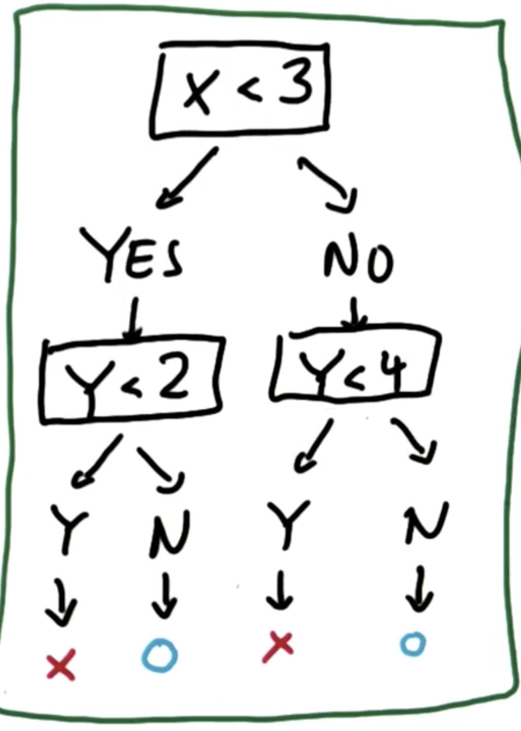
决策树利用如上图所示的树结构进行决策,每一个非叶子节点是一个判断条件,每一个叶子节点是结论。从跟节点开始,经过多次判断得出结论。
举个例子
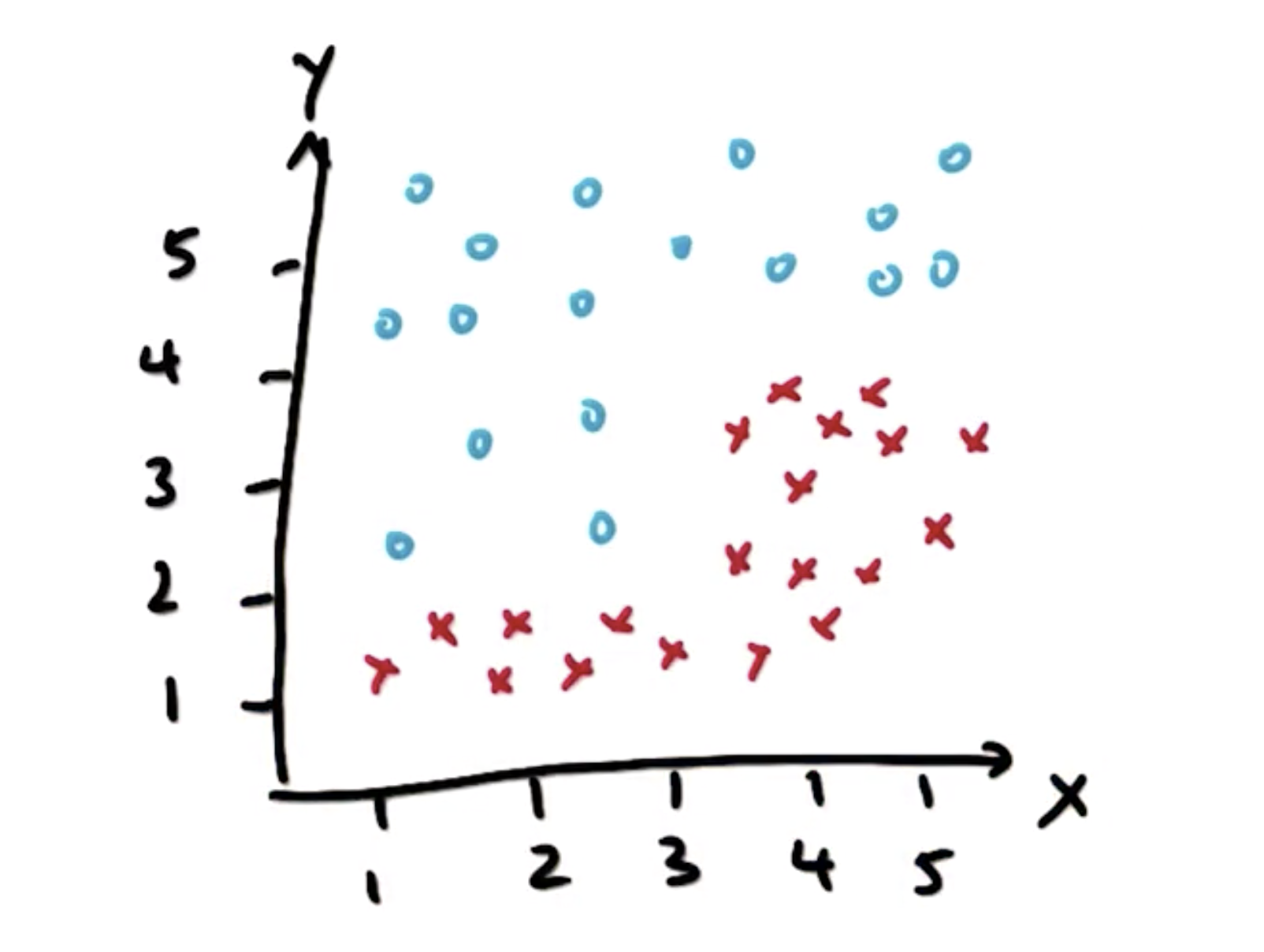
如图,利用决策树将两类样本点分类。
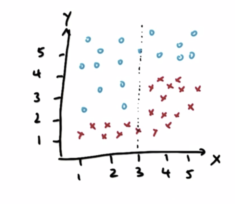
先从X轴观察,在X = 3时,样本点有一次明显的“突变”,我们以X = 3作为一次决策,进行一次划分:
再从Y轴观察,两类样本点在Y = 4 和Y = 2处可以进行划分,进而进行两次划分:
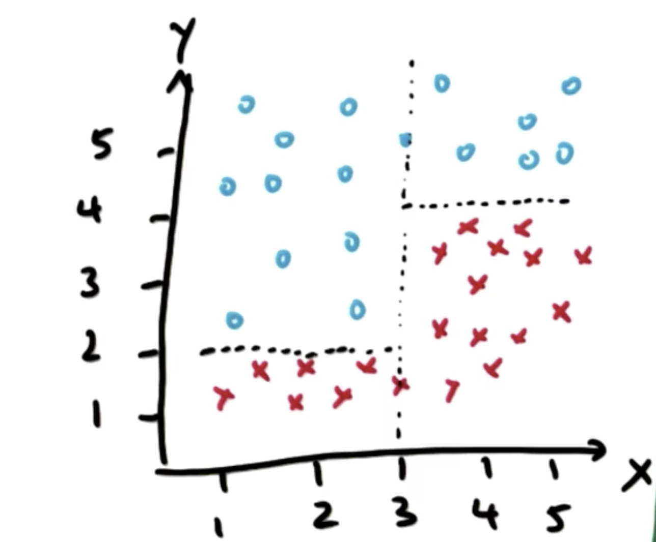
通过这几次划分,样本点被划分为四个部分,其中两类样本点各划为两部分,而且无法再继续分割,这种分割的过程就是决策树:
- 熵(entropy)
熵的作用:用于控制决策树在什么条件下做出决策,即在什么条件下分割数据
熵的定义:它是一系列样本中的不纯度的测量值(measure of impurity in a bunch of examples)
建立决策树的过程就是找到变量划分点从而产生尽可能的单一的子集,实际上决策树做决策的过程,就是对这个过程的递归重复。
熵描述了数据的混乱程度,熵越大,混乱程度越高,也就是纯度越低;反之,熵越小,混乱程度越低,纯度越高。 熵的计算公式如下所示:
其中Pi表示类i的数量占比。以二分类问题为例,如果两类的数量相同,此时分类节点的纯度最低,熵等于1;如果节点的数据属于同一类时,此时节点的纯度最高,熵等于0。
熵的最大值为1,最小值为0
- 信息增益
用信息增益表示分裂前后跟的数据复杂度和分裂节点数据复杂度的变化值,计算公式表示为:
其中Gain表示节点的复杂度,Gain越高,说明复杂度越高。信息增益也可以说是分裂前的熵减去孩子节点的熵的和,信息增益越大,分裂后的熵减小得越多,分类的效果越明显。
- 偏差(bias)与方差(variance)
高偏差机器学习算法实际上会忽略训练数据,它几乎没有能力学习任何数据,这被称为偏差。
另一个极端情况就是高方差,它只能复现曾经出现过的东西,对于没有出现过的情况,他的反应非常差。
通过调整参数让偏差与方差平衡,使算法具有一定泛化能力,但仍然对训练数据开放,能根据数据调整模型,是机器学习的要点。
- 代码实现
环境:MacOS mojave 10.14.3
Python 3.7.0
使用库:scikit-learn 0.19.2
sklearn.tree官方库:https://scikit-learn.org/stable/modules/tree.html
>>> from sklearn import tree
>>> X = [[0, 0], [1, 1]]    #两个样本点
>>> Y = [0, 1]                #分别属于两个标签
>>> clf = tree.DecisionTreeClassifier()    #进行分类
>>> clf = clf.fit(X, Y)
>>> clf.predict([[2., 2.]])   #预测新点
array([1])                        #新点通过分类属于标签1
Main.py 主程序
import sys
from class_vis import prettyPicture, output_image
from prep_terrain_data import makeTerrainData

import matplotlib.pyplot as plt
import numpy as np
import pylab as pl
from classifyDT import classify

features_train, labels_train, features_test, labels_test = makeTerrainData()


### the classify() function in classifyDT is where the magic
### happens--fill in this function in the file 'classifyDT.py'!
clf = classify(features_train, labels_train)


#### grader code, do not modify below this line

prettyPicture(clf, features_test, labels_test)
accuracy = clf.score(features_test, labels_test)

# output_image("test.png", "png", open("test.png", "rb").read())
print (accuracy)
acc = accuracy    ### you fill this in!
classifyDT.py 决策树分类
def classify(features_train, labels_train):

    ### your code goes here--should return a trained decision tree classifer
    from sklearn.tree import DecisionTreeClassifier
    clf = DecisionTreeClassifier(random_state=0)
    clf.fit(features_train,labels_train)


    return clf
perp_terrain_data.py 生成训练点
import random


def makeTerrainData(n_points=1000):
###############################################################################
### make the toy dataset
    random.seed(42)
    grade = [random.random() for ii in range(0,n_points)]
    bumpy = [random.random() for ii in range(0,n_points)]
    error = [random.random() for ii in range(0,n_points)]
    y = [round(grade[ii]*bumpy[ii]+0.3+0.1*error[ii]) for ii in range(0,n_points)]
    for ii in range(0, len(y)):
        if grade[ii]>0.8 or bumpy[ii]>0.8:
            y[ii] = 1.0

### split into train/test sets
    X = [[gg, ss] for gg, ss in zip(grade, bumpy)]
    split = int(0.75*n_points)
    X_train = X[0:split]
    X_test  = X[split:]
    y_train = y[0:split]
    y_test  = y[split:]

    grade_sig = [X_train[ii][0] for ii in range(0, len(X_train)) if y_train[ii]==0]
    bumpy_sig = [X_train[ii][1] for ii in range(0, len(X_train)) if y_train[ii]==0]
    grade_bkg = [X_train[ii][0] for ii in range(0, len(X_train)) if y_train[ii]==1]
    bumpy_bkg = [X_train[ii][1] for ii in range(0, len(X_train)) if y_train[ii]==1]

#    training_data = {"fast":{"grade":grade_sig, "bumpiness":bumpy_sig}
#            , "slow":{"grade":grade_bkg, "bumpiness":bumpy_bkg}}


    grade_sig = [X_test[ii][0] for ii in range(0, len(X_test)) if y_test[ii]==0]
    bumpy_sig = [X_test[ii][1] for ii in range(0, len(X_test)) if y_test[ii]==0]
    grade_bkg = [X_test[ii][0] for ii in range(0, len(X_test)) if y_test[ii]==1]
    bumpy_bkg = [X_test[ii][1] for ii in range(0, len(X_test)) if y_test[ii]==1]

    test_data = {"fast":{"grade":grade_sig, "bumpiness":bumpy_sig}
            , "slow":{"grade":grade_bkg, "bumpiness":bumpy_bkg}}

    return X_train, y_train, X_test, y_test
#    return training_data, test_data
class_vis.py 绘图与保存图像
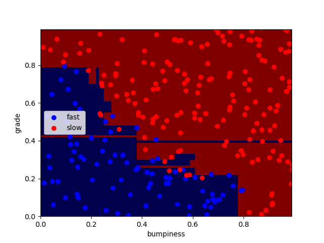
import warnings
warnings.filterwarnings("ignore")

import matplotlib
matplotlib.use('agg')

import matplotlib.pyplot as plt
import pylab as pl
import numpy as np

#import numpy as np
#import matplotlib.pyplot as plt
#plt.ioff()

def prettyPicture(clf, X_test, y_test):
    x_min = 0.0; x_max = 1.0
    y_min = 0.0; y_max = 1.0

    # Plot the decision boundary. For that, we will assign a color to each
    # point in the mesh [x_min, m_max]x[y_min, y_max].
    h = .01  # step size in the mesh
    xx, yy = np.meshgrid(np.arange(x_min, x_max, h), np.arange(y_min, y_max, h))
    Z = clf.predict(np.c_[xx.ravel(), yy.ravel()])

    # Put the result into a color plot
    Z = Z.reshape(xx.shape)
    plt.xlim(xx.min(), xx.max())
    plt.ylim(yy.min(), yy.max())

    plt.pcolormesh(xx, yy, Z, cmap=pl.cm.seismic)

    # Plot also the test points
    grade_sig = [X_test[ii][0] for ii in range(0, len(X_test)) if y_test[ii]==0]
    bumpy_sig = [X_test[ii][1] for ii in range(0, len(X_test)) if y_test[ii]==0]
    grade_bkg = [X_test[ii][0] for ii in range(0, len(X_test)) if y_test[ii]==1]
    bumpy_bkg = [X_test[ii][1] for ii in range(0, len(X_test)) if y_test[ii]==1]

    plt.scatter(grade_sig, bumpy_sig, color = "b", label="fast")
    plt.scatter(grade_bkg, bumpy_bkg, color = "r", label="slow")
    plt.legend()
    plt.xlabel("bumpiness")
    plt.ylabel("grade")

    plt.savefig("test.png")
得到结果,正确率90.8%

其中,狭长区域为过拟合
- 决策树的参数
min_samples_split可分割的样本数量下限,默认值为2
对于决策树最下层的每一个节点,是否还要继续分割,min_samples_split决定了能够继续进行分割的最少分割样本
acc_min_samples.py acc_min_samples对比
import sys
from class_vis import prettyPicture
from prep_terrain_data import makeTerrainData

import matplotlib.pyplot as plt
import numpy as np
import pylab as pl

features_train, labels_train, features_test, labels_test = makeTerrainData()


########################## DECISION TREE #################################


### your code goes here--now create 2 decision tree classifiers,
### one with min_samples_split=2 and one with min_samples_split=50
### compute the accuracies on the testing data and store
### the accuracy numbers to acc_min_samples_split_2 and
### acc_min_samples_split_50, respectively


from sklearn.tree import DecisionTreeClassifier
clf1 = DecisionTreeClassifier(min_samples_split=2)
clf2 = DecisionTreeClassifier(min_samples_split=50)

clf1.fit(features_train,labels_train)
clf2.fit(features_train,labels_train)

acc_min_samples_split_2 = clf1.score(features_test, labels_test)
acc_min_samples_split_50 = clf2.score(features_test, labels_test)


print (acc_min_samples_split_2)
print (acc_min_samples_split_50)

#choose one of two
prettyPicture(clf1, features_test, labels_test)
# prettyPicture(clf2, features_test, labels_test)

上图,min_samples_split分别为2 和50
得到正确率分别为90.8%和91.2%
- 决策树的优点与缺点
易于使用,易于理解
容易过拟合,尤其对于具有包含大量特征的数据时,复杂的决策树可能会过拟合数据,通过仔细调整参数,避免过拟合(对于节点上只有单个数据点的决策树,几乎肯定是过拟合)

 浙公网安备 33010602011771号