Einfuehrung in die Kuenstliche Intelligenz学习笔记
1.Uninformed Search
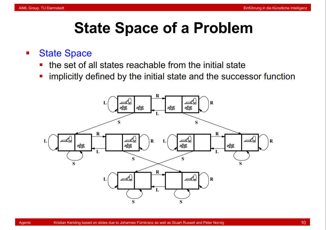
1.1 State Space of a Problem
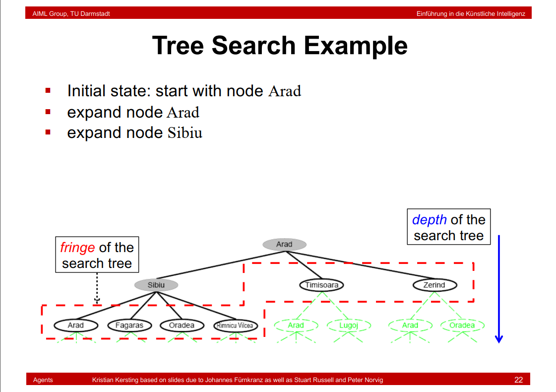
1.2 depth of the search tree and fringe of the search tree
1.3 States vs. Nodes

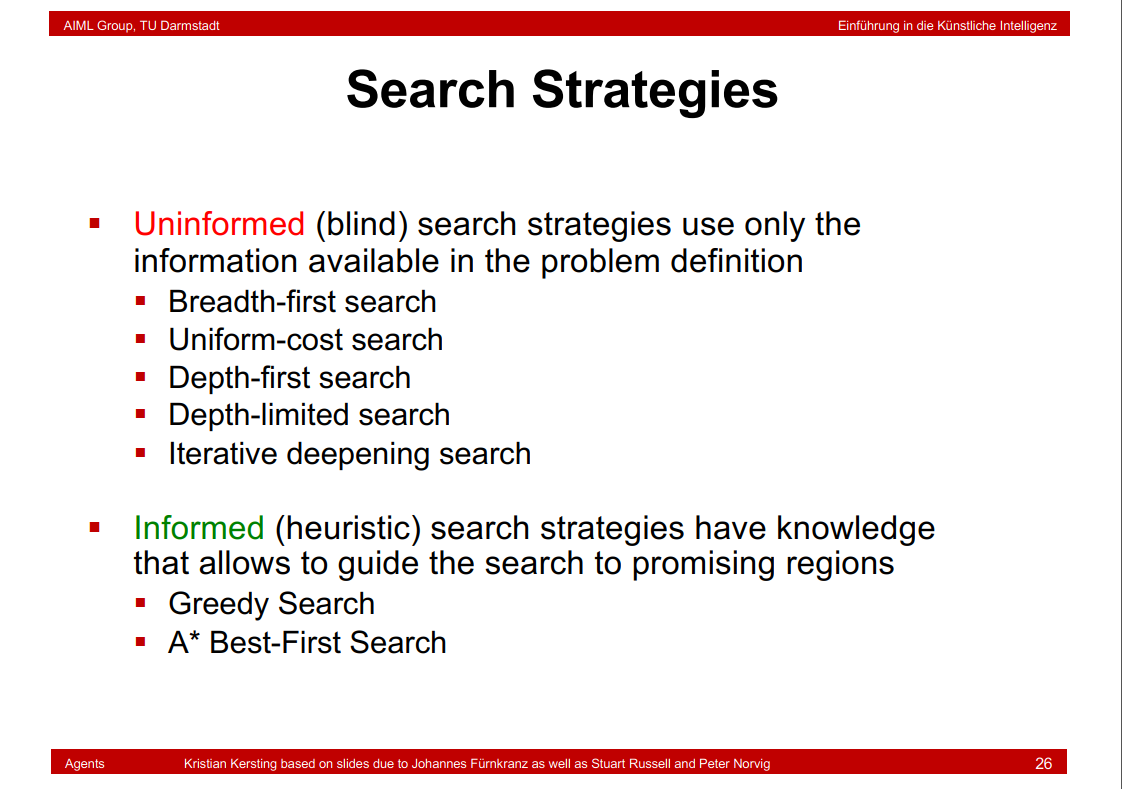
1.4 Search Strategies
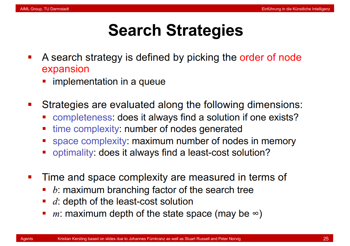
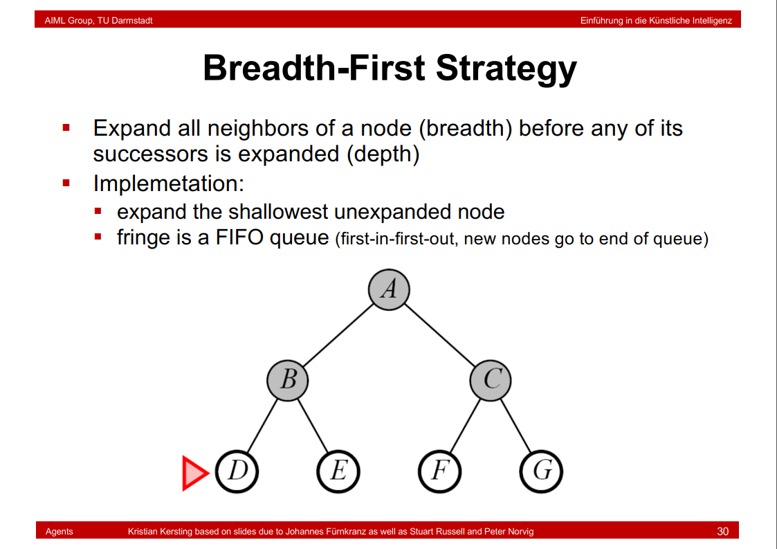
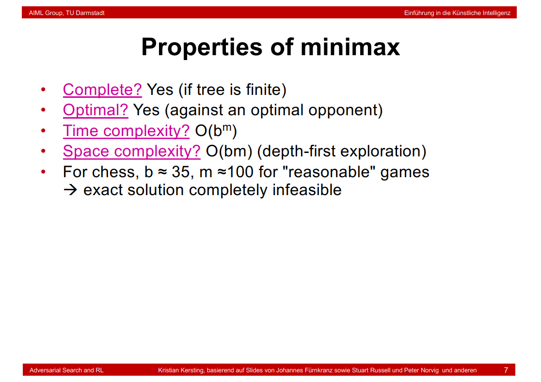
§ completeness: does it always find a solution if one exists?
§ time complexity: number of nodes generated
§ space complexity: maximum number of nodes in memory
§ optimality: does it always find a least-cost solution?
1.5 Breadth-First Strategy
1.6 Properties of Breadth-First Search
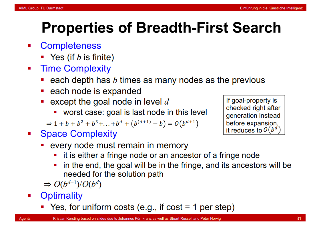
这里是一般情况b叉树,深度d从开始。Time complexity is the number of nodes. You need to traverse all nodes.
Space complexity is the same as well,since at worst case you need to hold all vertices in the queue.时间和空间复杂度都是结点的数量。
时间和空间复杂度为O(b^(d+1))。
时间复杂度最后一项是b^(d+1)-b = (\(b^d\) -1)* b = \(b^{d+1}\) - b
1.7 Uniform-Cost Search

时间和空间复杂度一致,为b^ (1+O(C^* /ε)); C^ *是最优代价,ε是每个步骤的最小代价;C^ */ε即是步骤数。
1.8 Depth-First Strategy
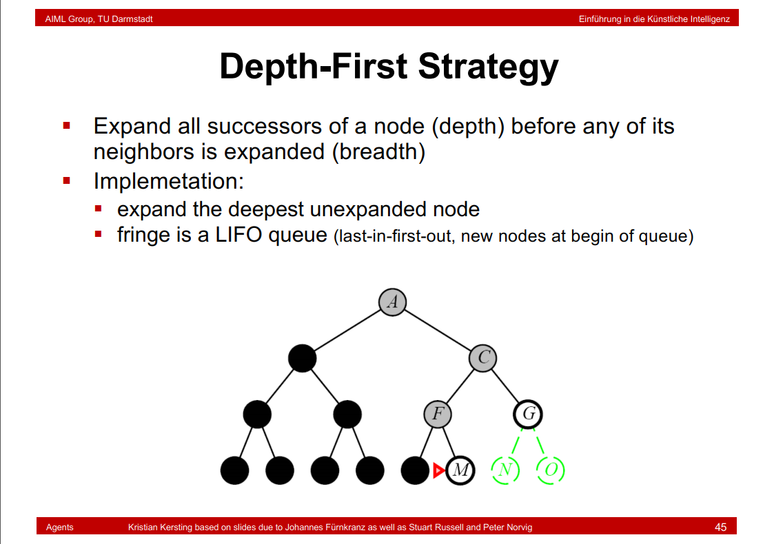
Expand all successors of a node (depth) before any of its
neighbors is expanded (breadth)
1.9 Properties of Depth-First Search
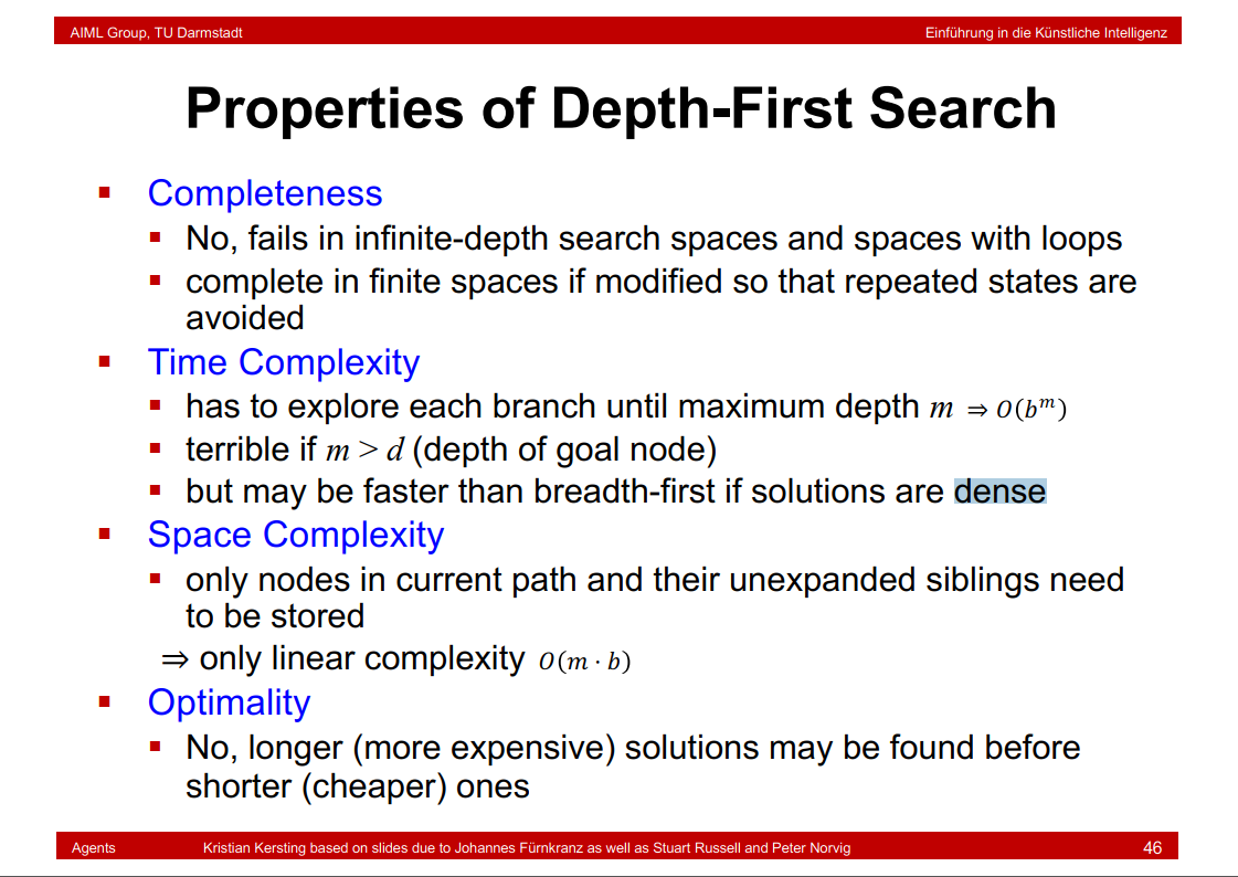
这里时间复杂度指的是平均时间复杂度,所以是O(b^m),空间复杂度指的是当前深度的总结点数,不包括同深度其他路径未展开的结点,所以是O(mb)
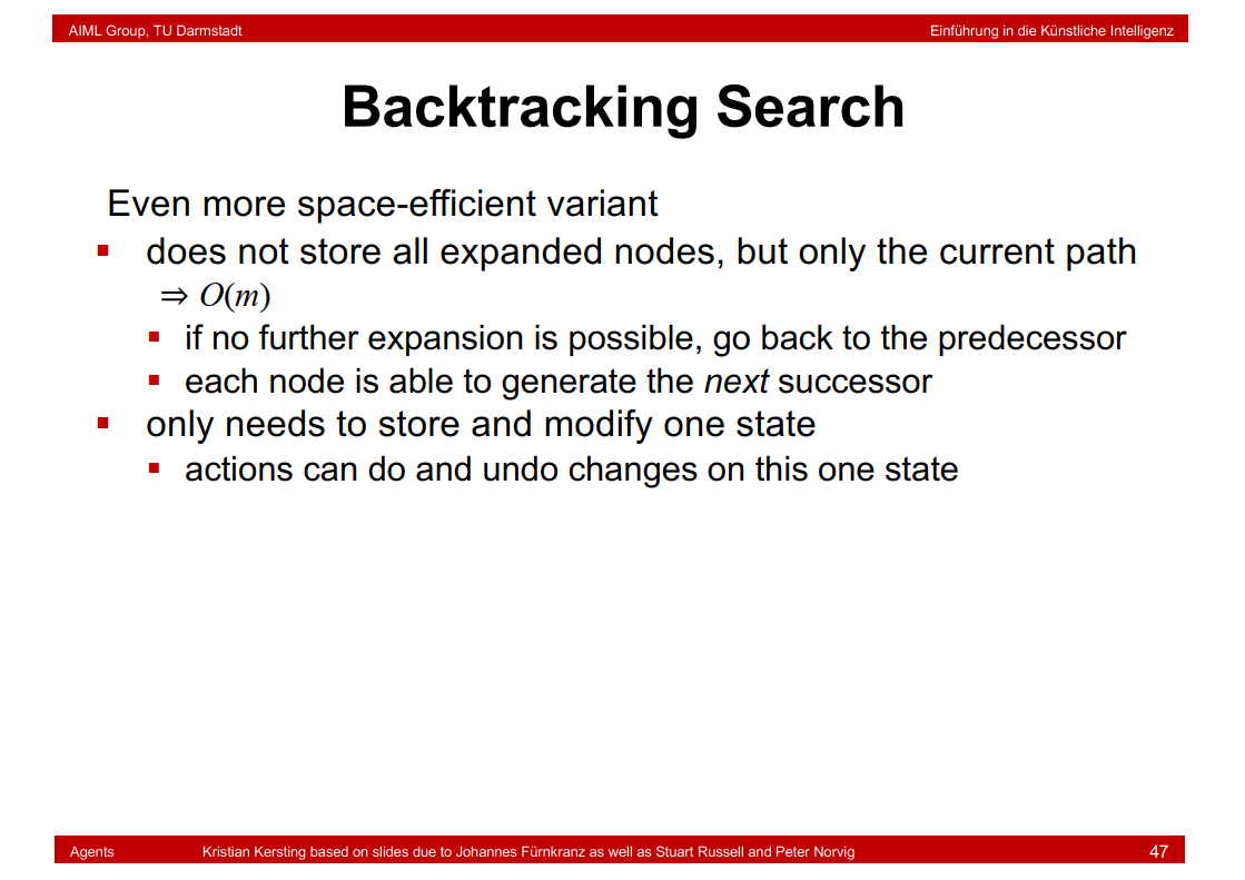
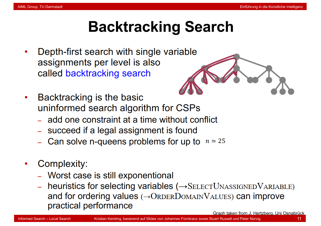
1.10 Backtracking Search
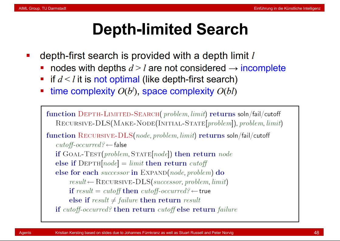
1.11 Depth-limited Search
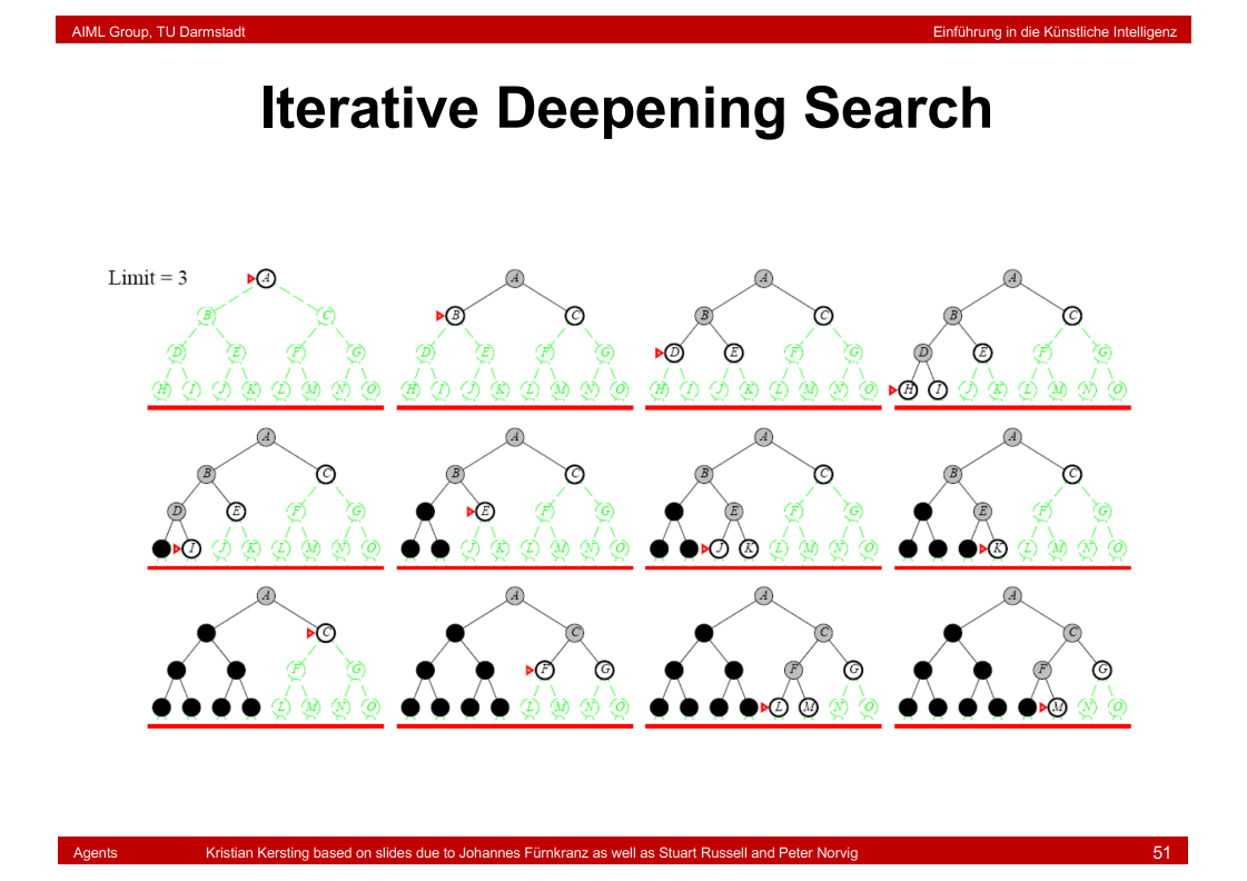
1.12 Iterative Deepening Search

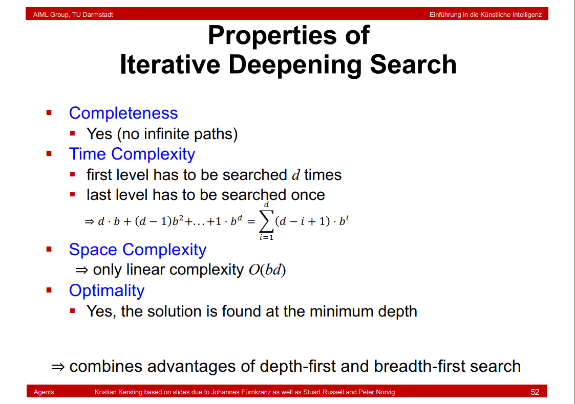
1.13 Properties of Iterative Deepening Search
参考:(https://zh.wikipedia.org/wiki/迭代深化深度优先搜索)
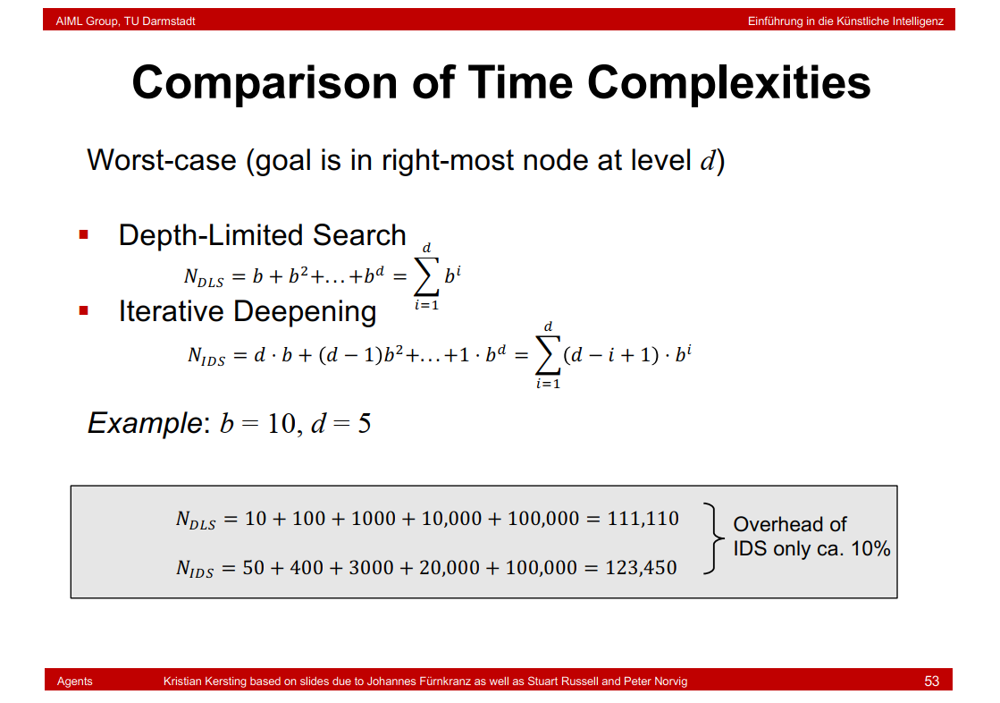
1.14 Comparison of Time Complexities of Depth-limited Search and Iterative Deepening Search
1.15 Bidirectional Search
双向搜索可以大大减少复杂度,b^(d/2) + b^(d/2) << b^d
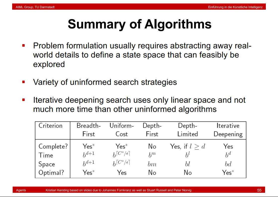
1.16 时间复杂度总结
2. Informed Search
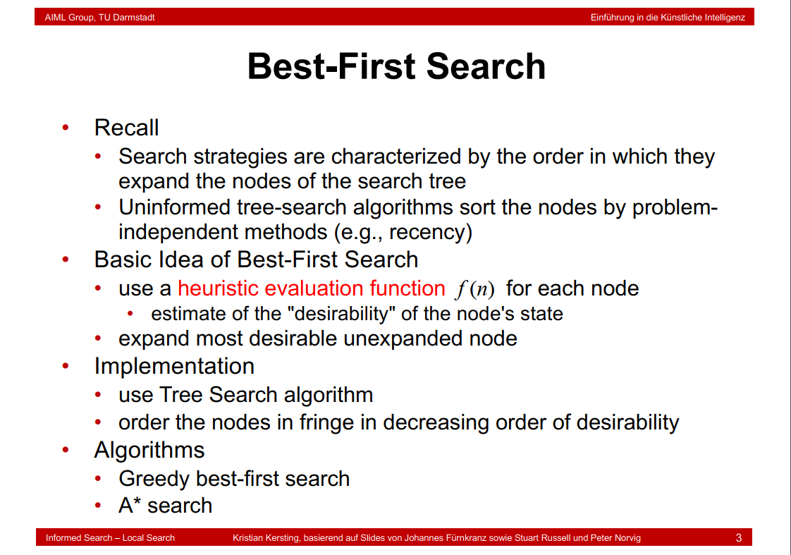
2.1 Best-First Search
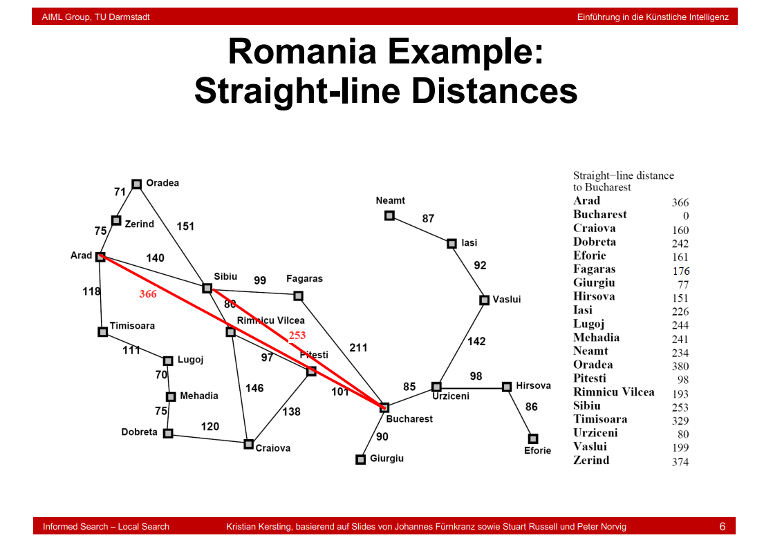
2.2 Romania Example: Straight-line Distances
2.3 Greedy Best-First Search
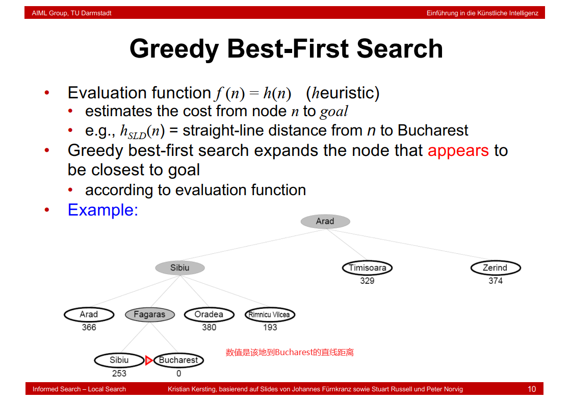
2.4 Properties of Greedy Best-First Search

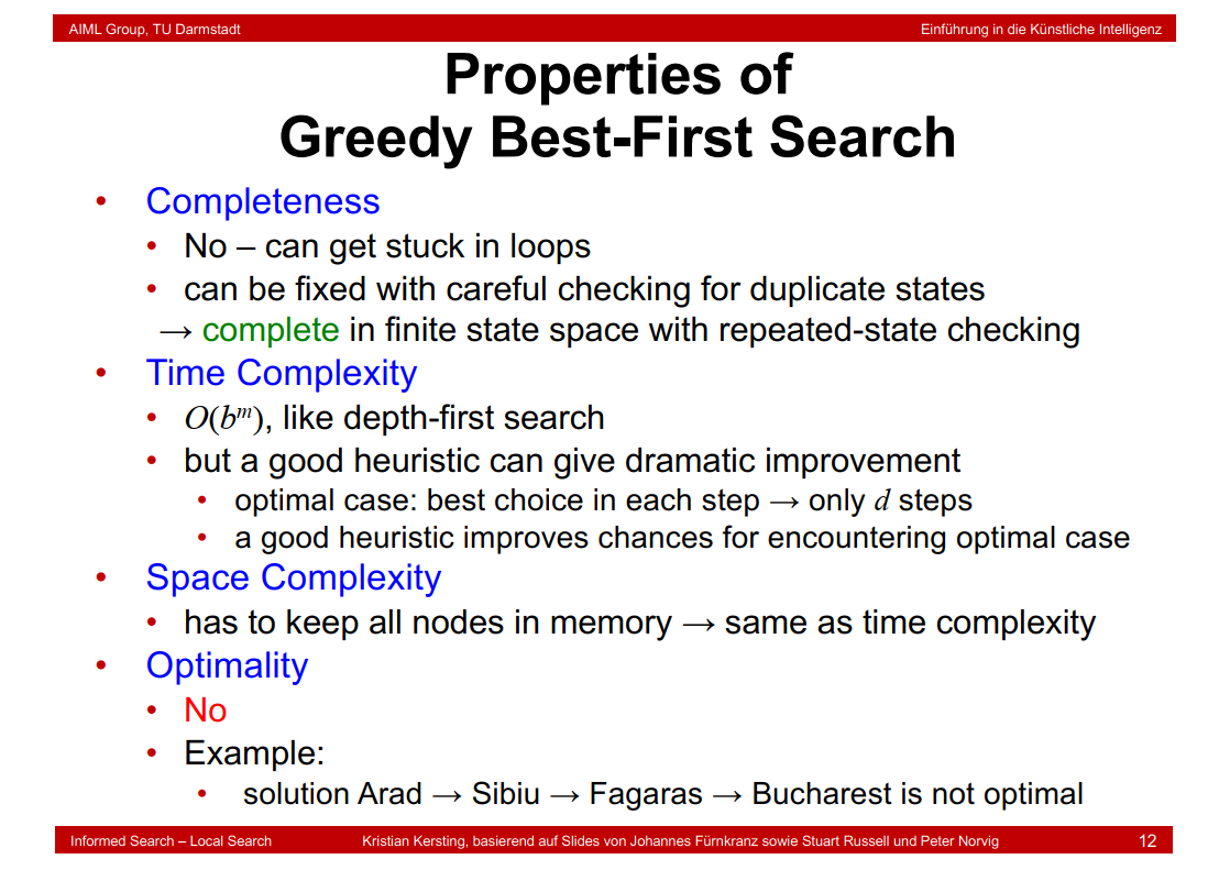
时间复杂度和空间复杂度与DFS一致。
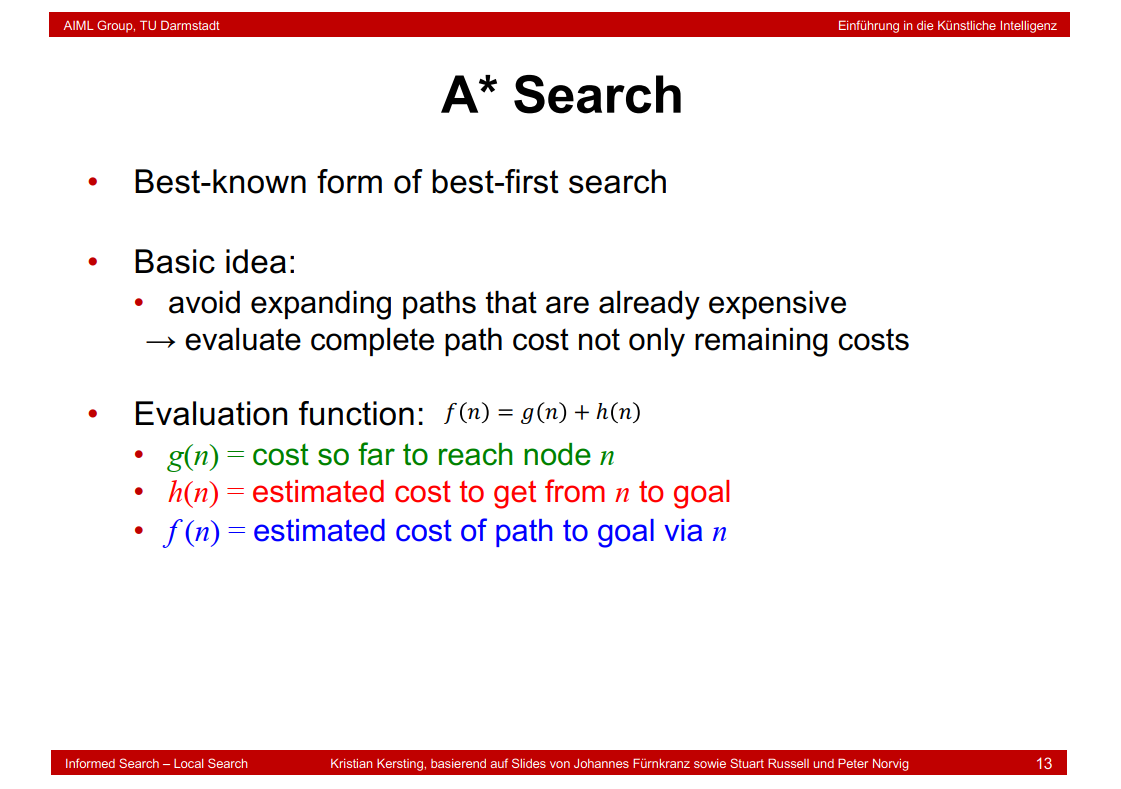
2.5 A* Search
2.6 Beispiel

2.7 A* Search Example


计算同理,这里有个错误,Pitesti的距离是317+98=415
2.8 Properties of A*
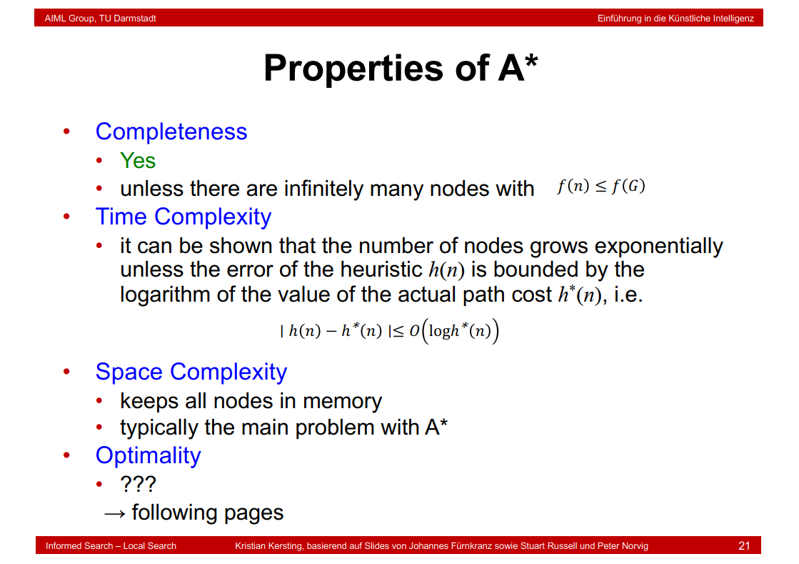
G应当是总结点数。
2.9 Admissible Heuristics

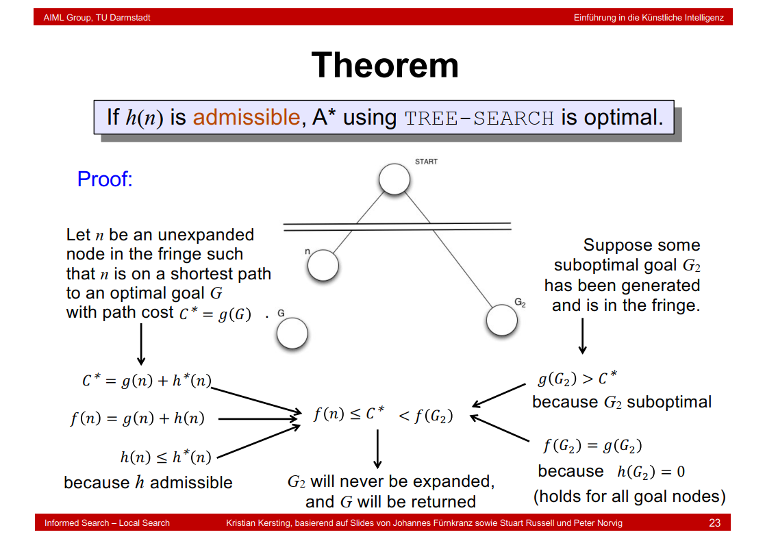
2.10 Theorem
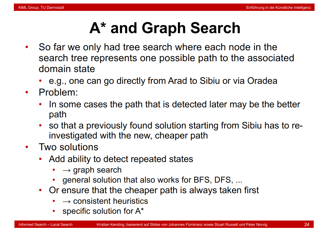
2.11 A* and Graph Search
在此算法中,如果以g(n)表示从起点到任意顶点n的实际距离,h(n)表示任意顶点n到目标顶点的估算距离(根据所采用的评估函数的不同而变化),h(n)为实际问题的代价值,那么A算法的估算函数为:
f(n)=g(n)+h(n)
这个公式遵循以下特性:
如果g(n)为0,即只计算任意顶点n到目标的评估函数h(n),而不计算起点到顶点n的距离,则算法转化为使用贪心策略的最良优先搜索,速度最快,但可能得不出最优解;
如果h(n)不大于顶点n到目标顶点的实际距离,则一定可以求出最优解,而且h(n)越小,需要计算的节点越多,算法效率越低;
如果h(n)为0,即只需求出起点到任意顶点n的最短路径g(n),而不计算任何评估函数h(n),则转化为单源最短路径问题,即Dijkstra算法,此时需要计算最多的顶点;
(https://blog.csdn.net/u013010889/article/details/78876377)
2.12 Repeated States
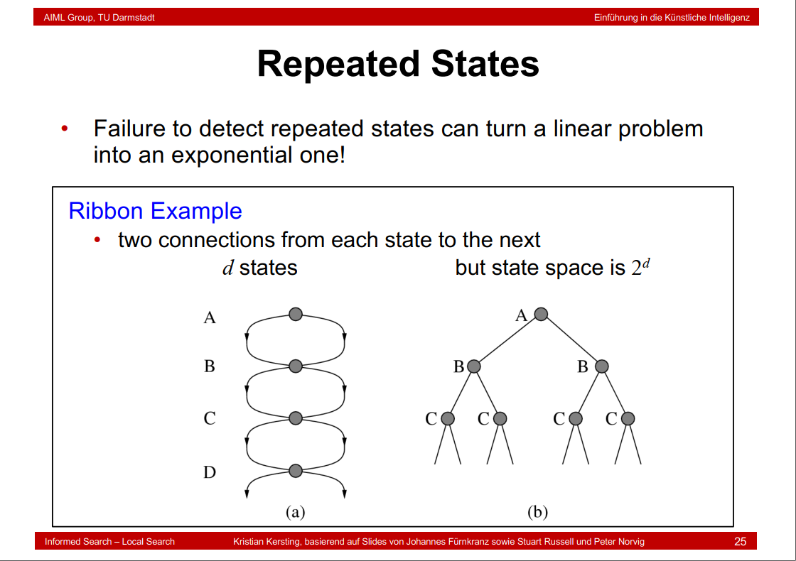
Repeated States是指重复访问结点,其会导致额外的开销。
b是a展开后的模样。
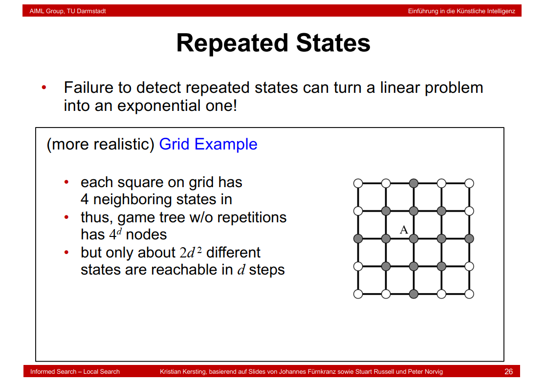
grid有四个子结点所以有时\(4^{d}\)结点。
\(2d^{2}\)证明过程:https://stackoverflow.com/questions/32303528/search-algorithm-with-avoiding-repeated-states
2.13 Consistent Heuristics

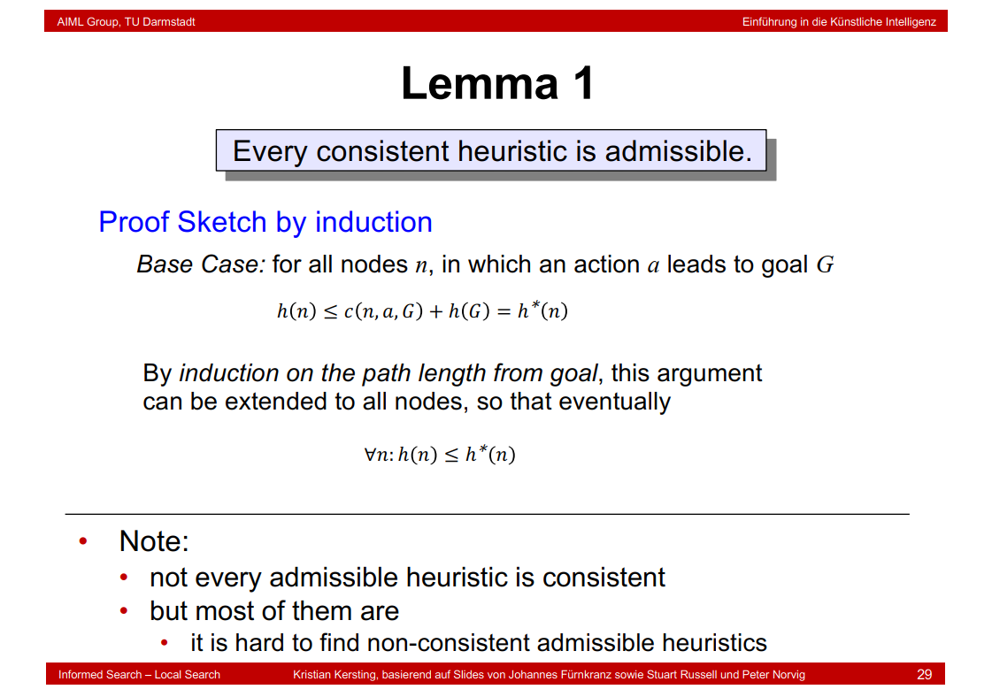
2.14 Lemma 1
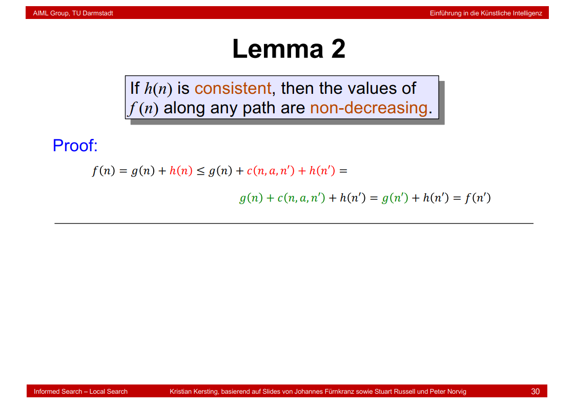
2.15 Lemma 2
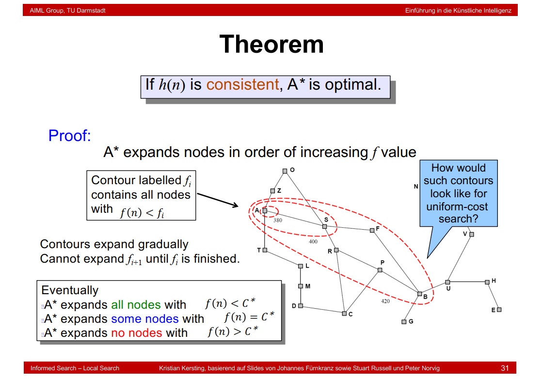
2.16 Theorem
2.17 Memory-Bounded Heuristic Search

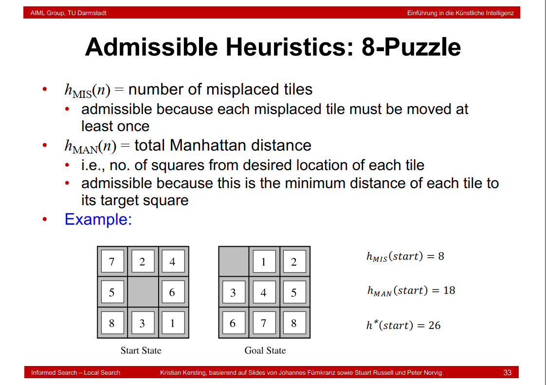
2.18 Admissible Heuristics: 8-Puzzle
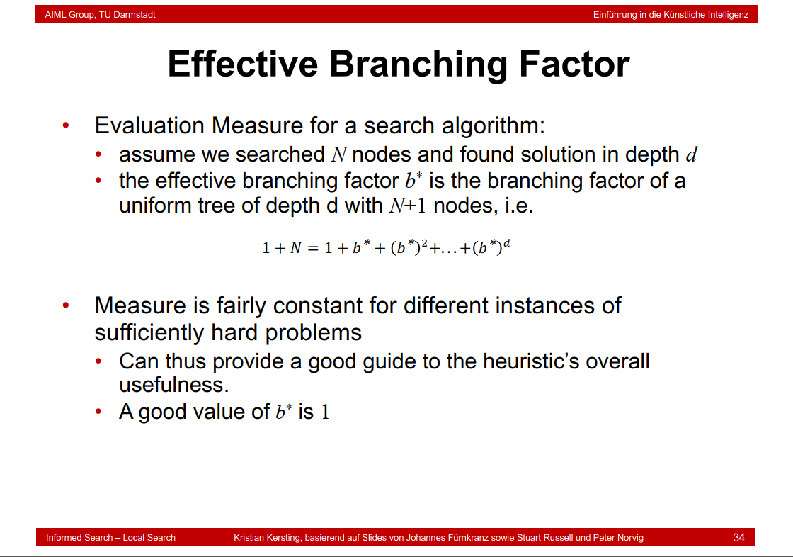
2.19 Effective Branching Factor
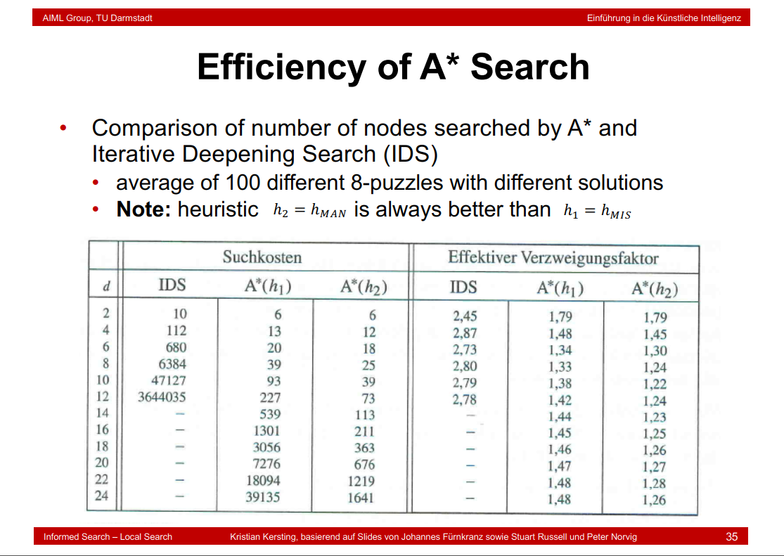
2.20 Efficiency of A* Search
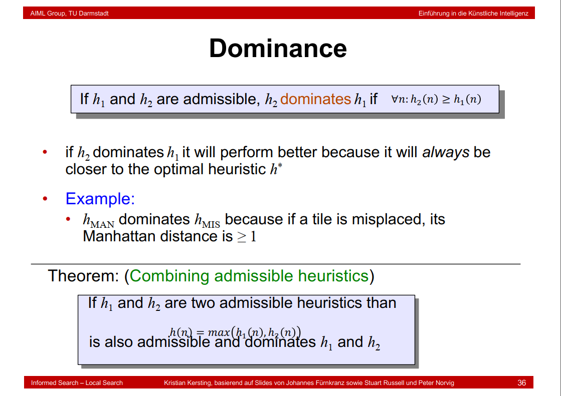
2.21 Dominance
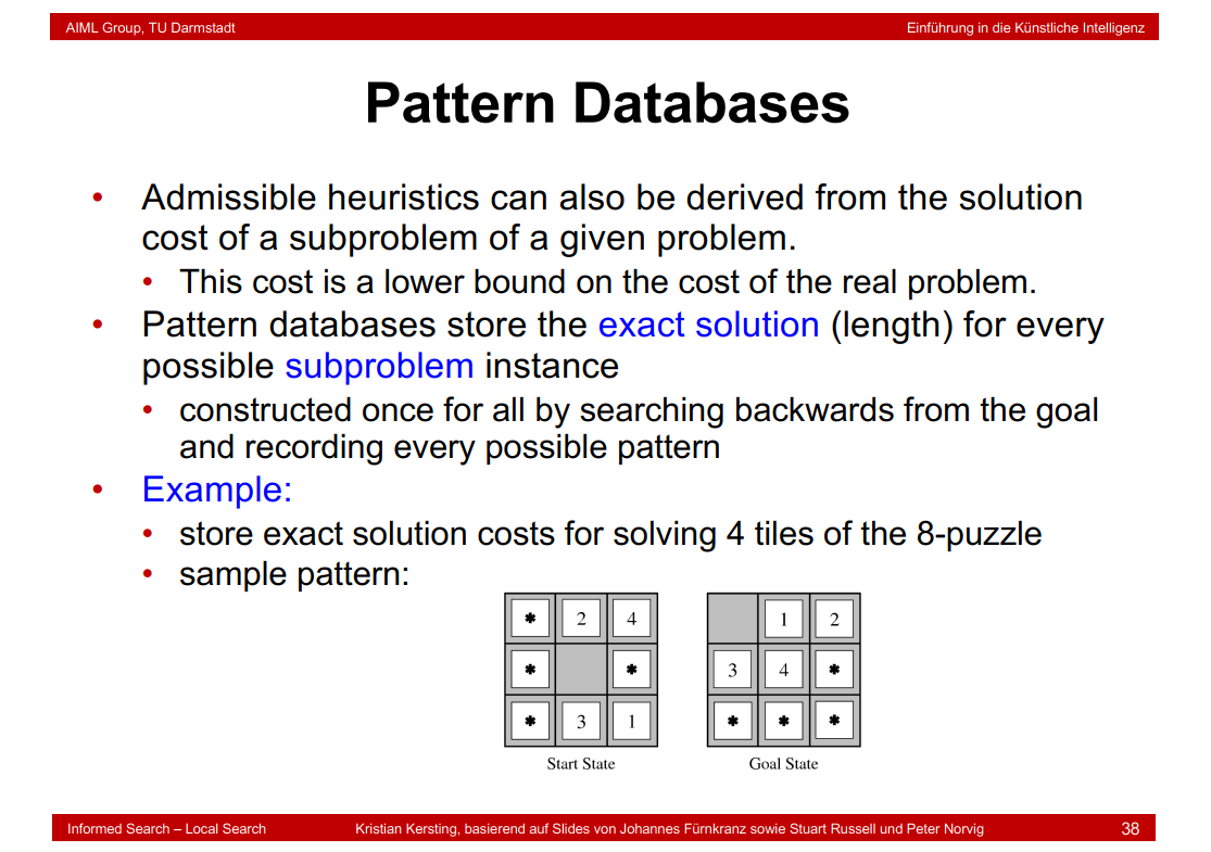
2.22 Pattern Databases
2.23 Summary

3. Search Local
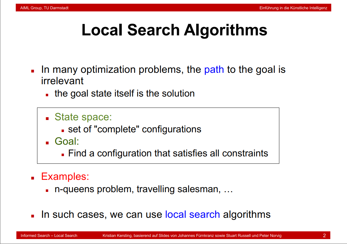
3.1 Local Search Algorithms
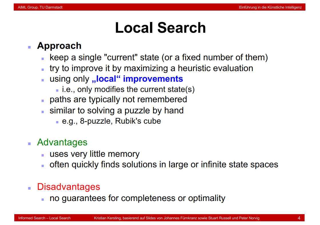
3.2 Local Search
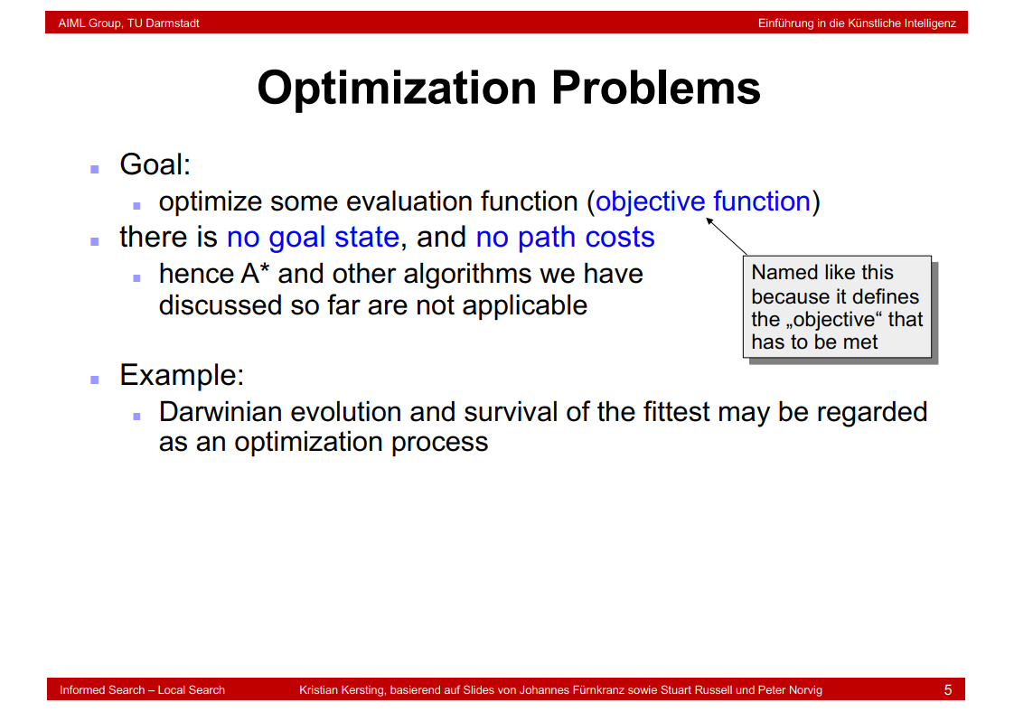
3.3 Optimization Problems
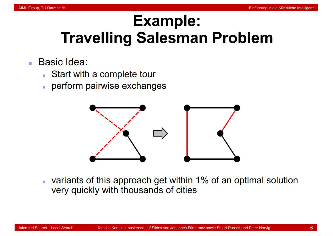
3.4 Example:Travelling Salesman Problem
3.5 Example: n-Queens Problem

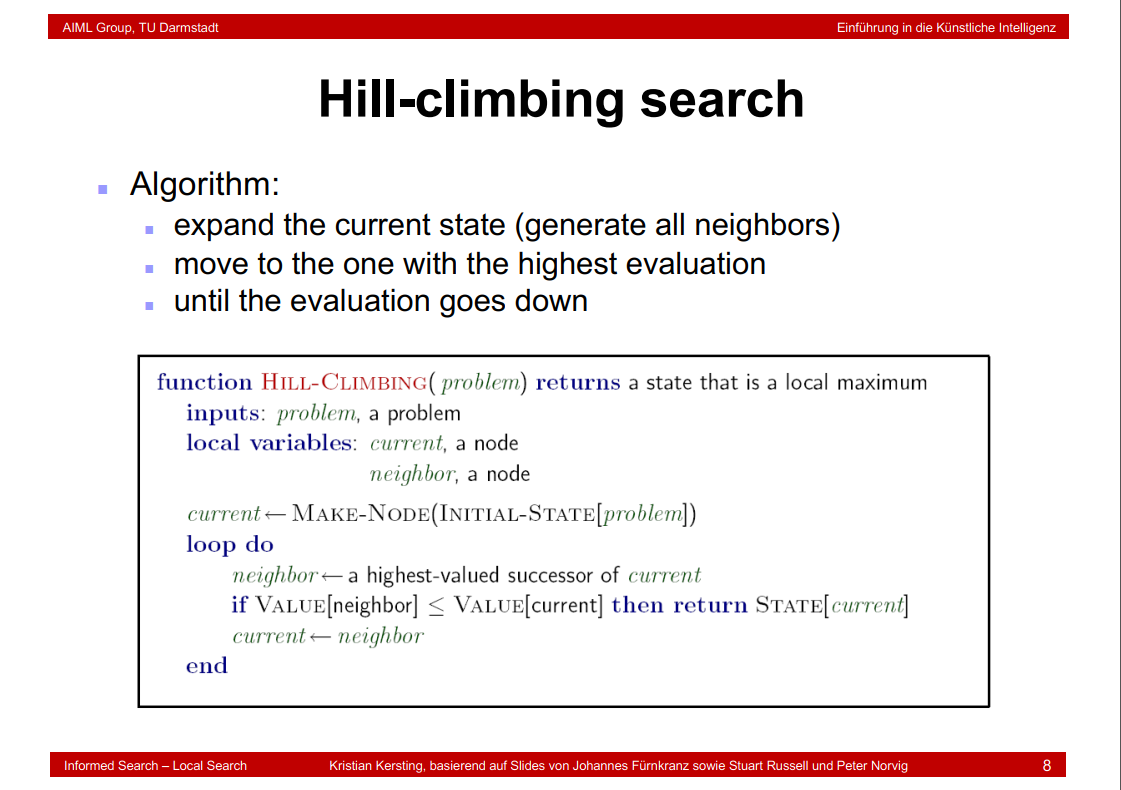
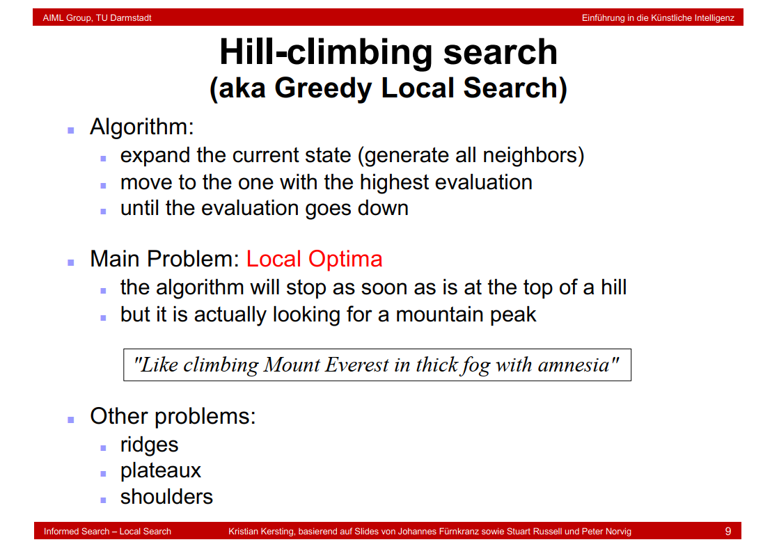
3.6 Hill-climbing search
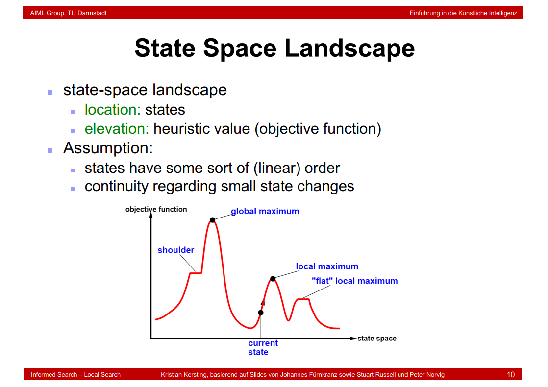
3.7 State Space Landscape
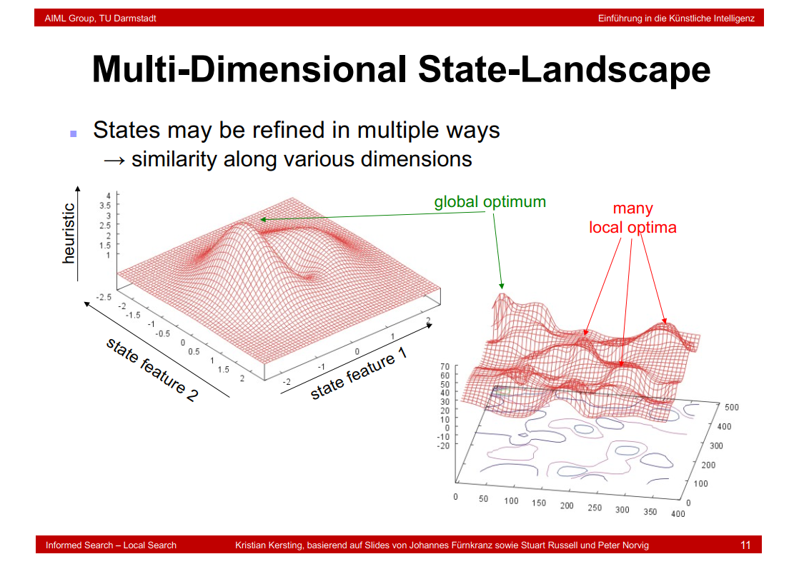
3.8 Multi-Dimensional State-Landscape
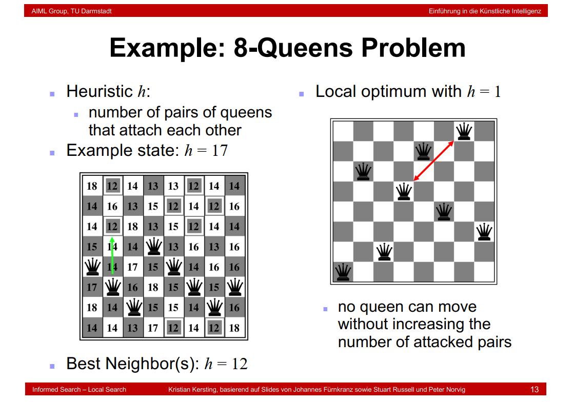
3.9 Example: 8-Queens Problem
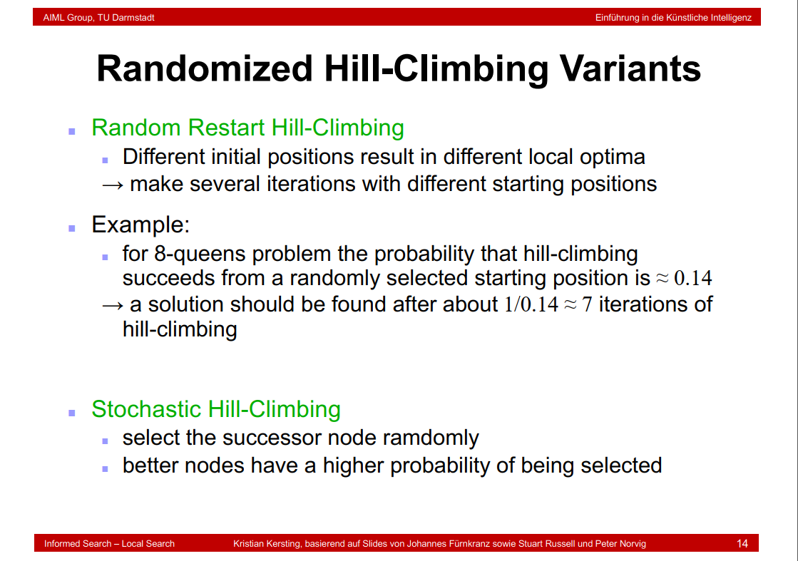
3.10 Randomized Hill-Climbing Variants
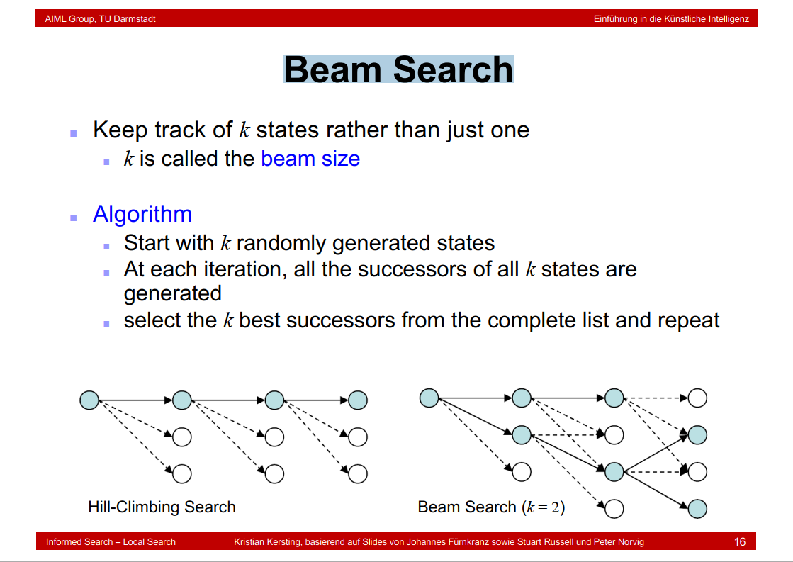
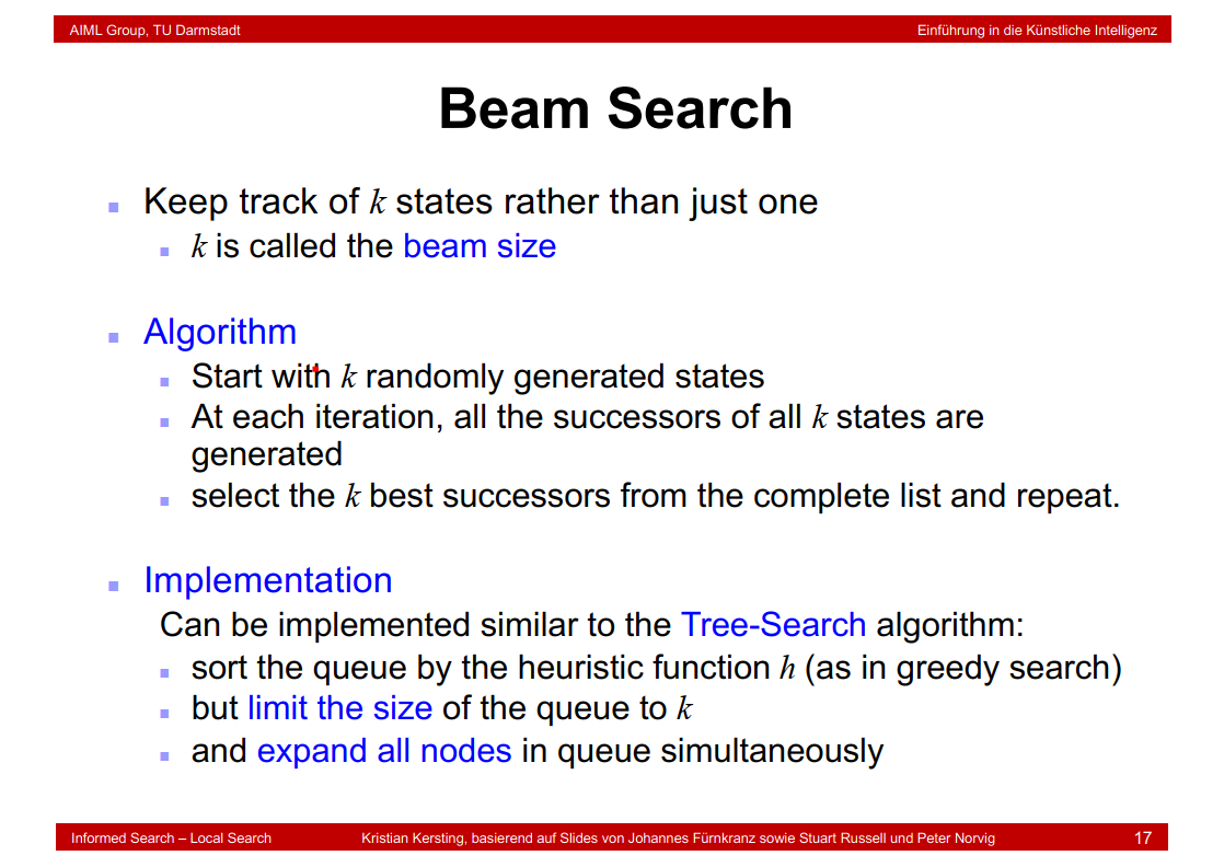
3.11 Beam Search

3.12 Simulated Annealing Search
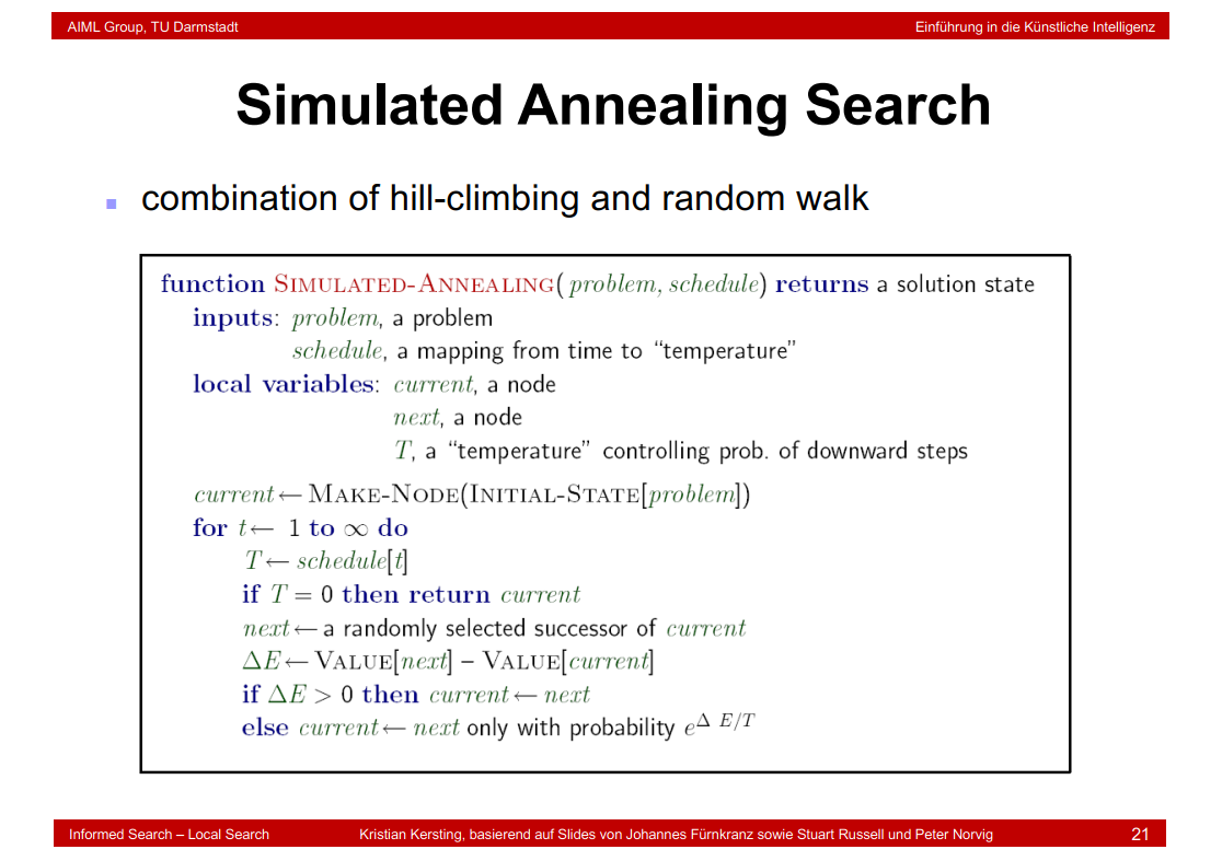
模拟退火算法是一种随机算法,并不一定能找到全局的最优解,可以比较快的找到问题的近似最优解。
大白话模拟退火算法
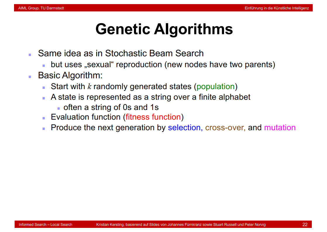
3.13 Genetic Algorithms
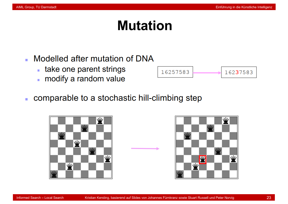
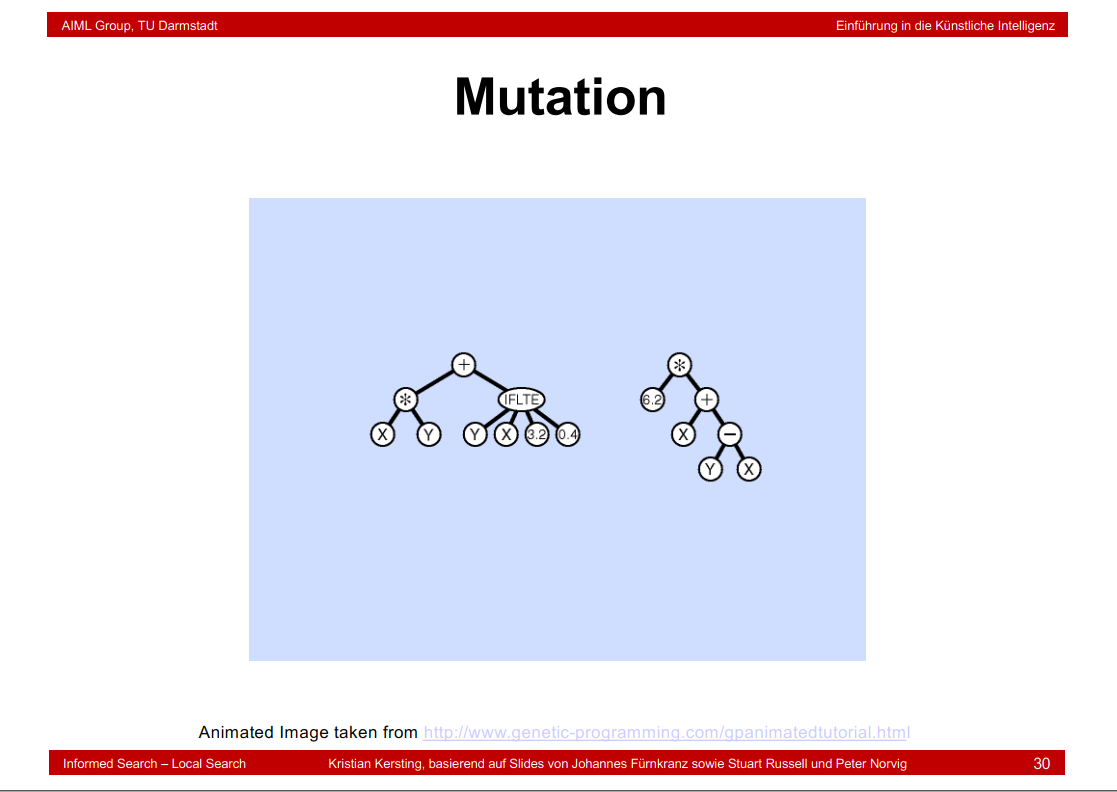
3.14 Mutation
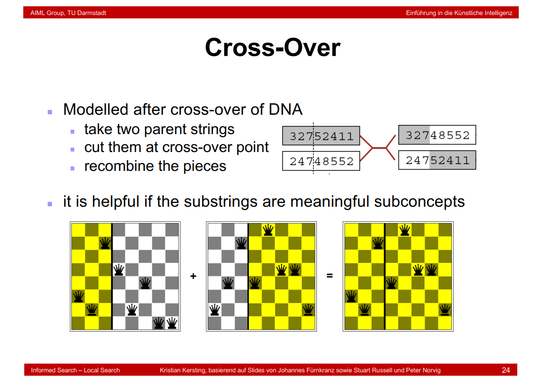
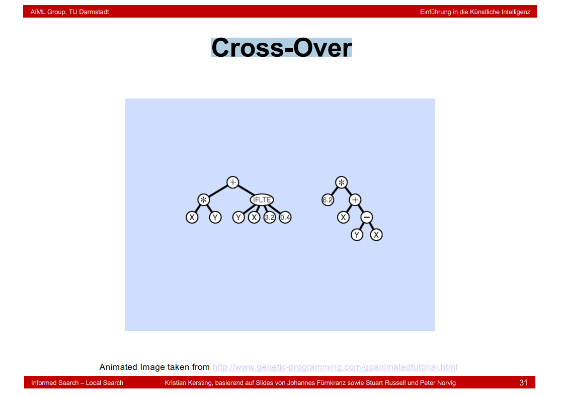
3.15 Cross-Over
Genetic Algorithms汇总:


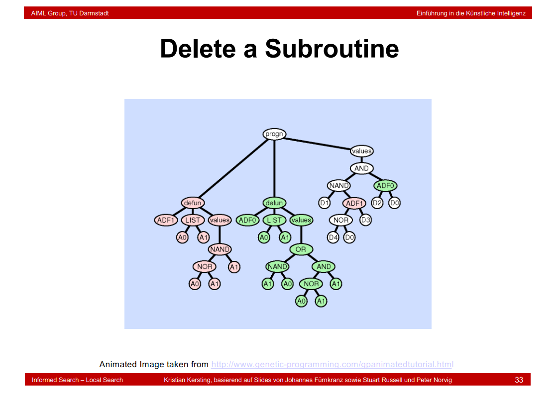
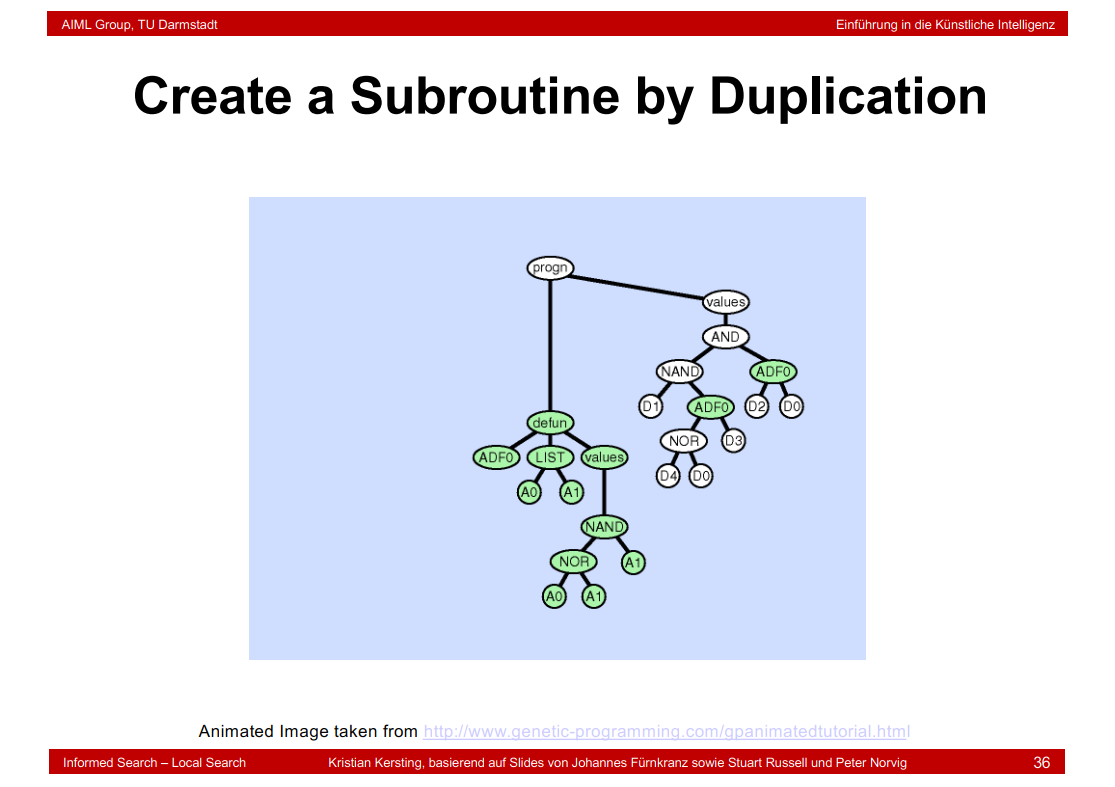
3.16 Genetic Programming
Random Initialization of Population:
Mutation:
Cross-Over:
Create a Subroutine:

Delete a Subroutine:
Duplicate an Argument:

Create a Subroutine by Duplication:
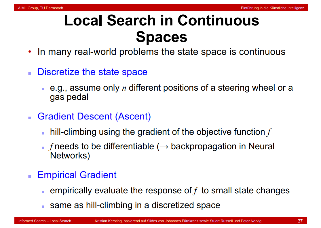
3.17 Local Search in Continuous Spaces
4.search constraints
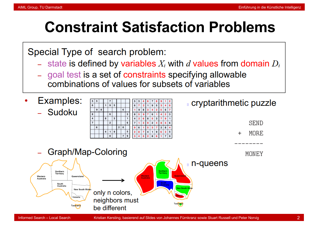
4.1 Constraint Satisfaction Problems
4.2 Constraint Graph

相邻的结点不能含有同样的颜色

\(X_{1}\),\(X_{2}\),\(X_{3}\)分别表示十位、百位和千位上的进位变量。
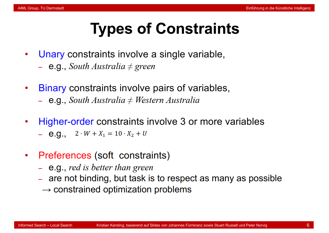
4.3 Types of Constraints
4.4 Solving CSP Problems

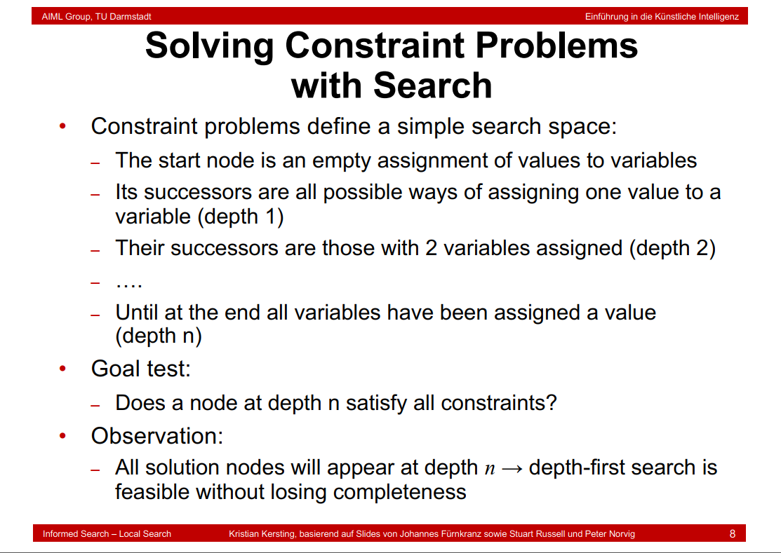
4.5 Solving Constraint Problems with Search
4.6 Complexity of Naive Search
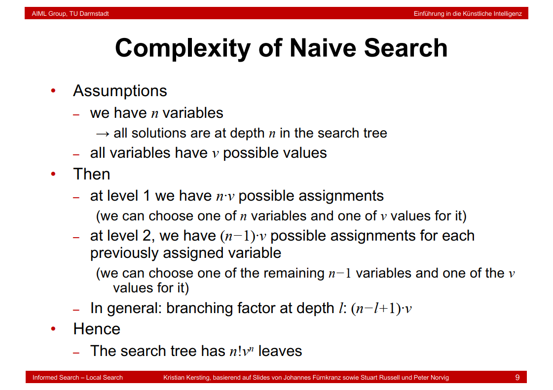
Naive Search的复杂度为nv(n-1)v..(n-l+1)v...*v = n!\(v^n\)
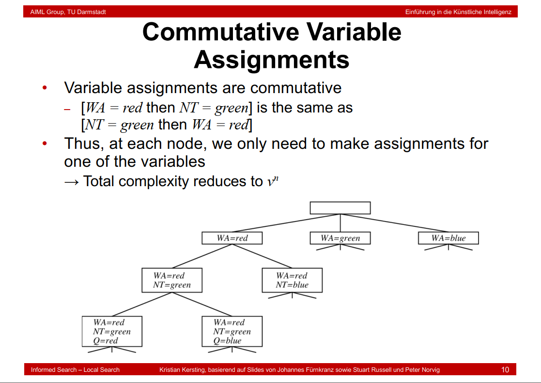
4.7 Commutative Variable Assignments
4.8 Backtracking Search

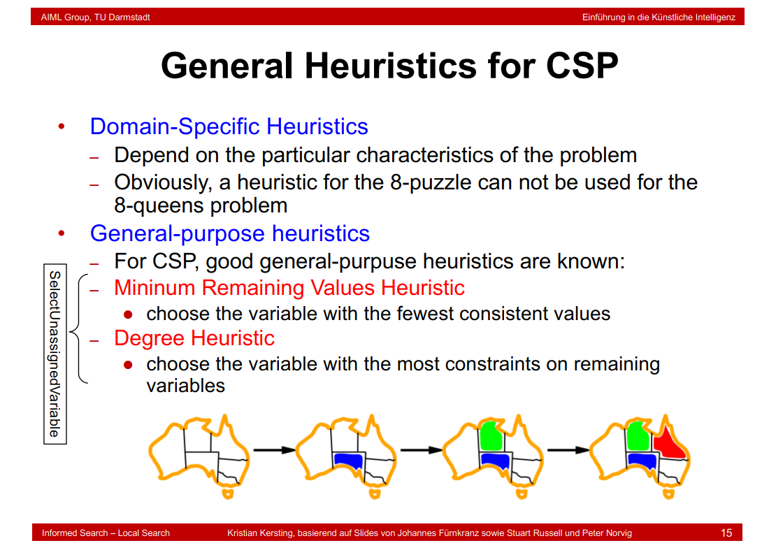
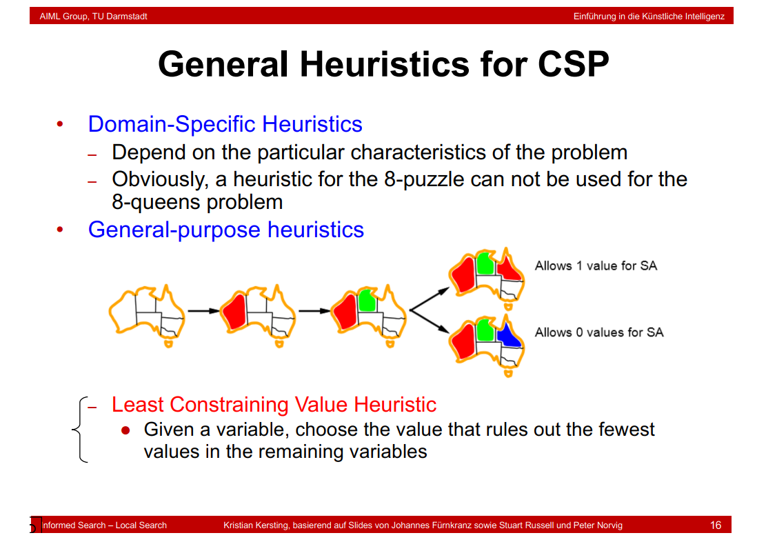
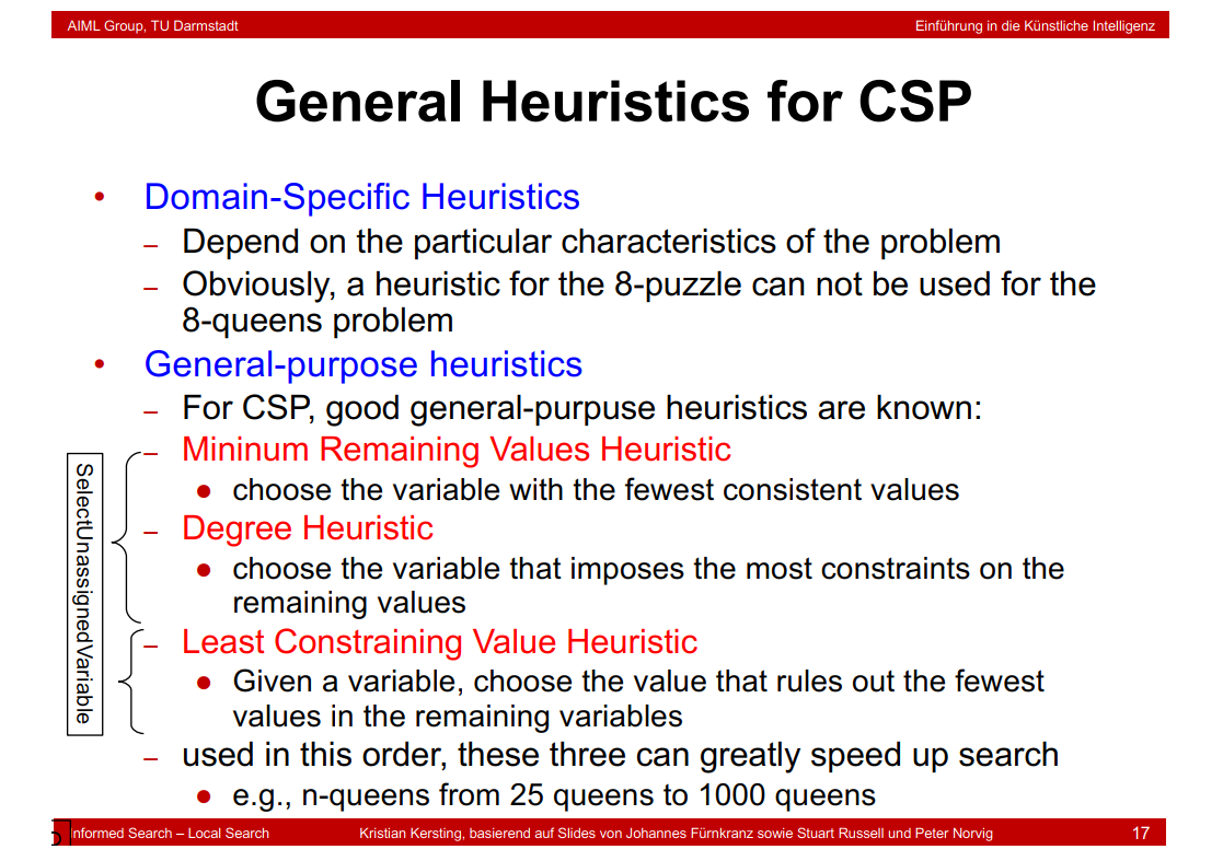
4.9 General Heuristics for CSP
4.10 Constraint Propagation - Sudoku
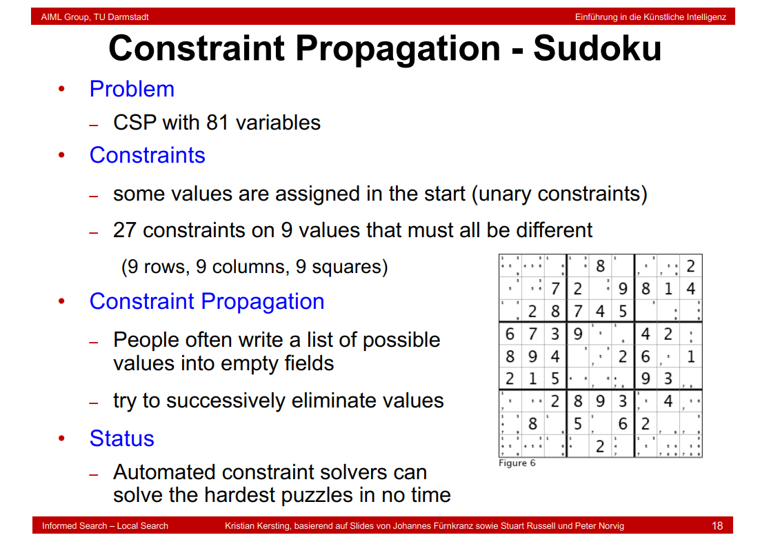
4.11 Node Consistency

4.12 Forward Checking
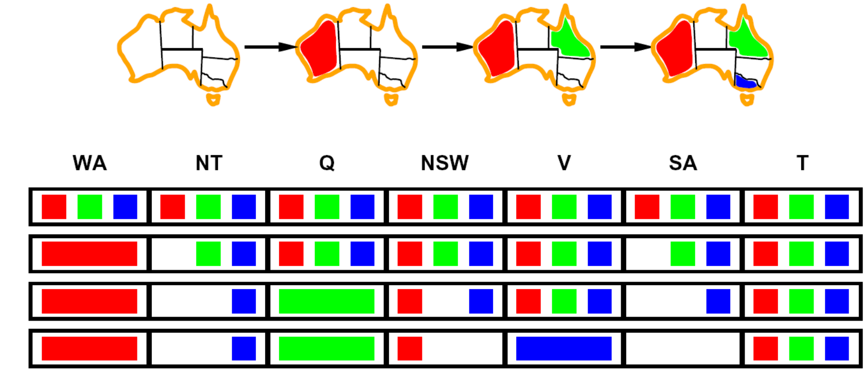
前向检验(Forward Checking):检查未分配变量的合法剩余值,当任何变量没有合法值时终止。
上图中,长条形颜色表示给对应地图上色,正方形颜色表示未上色,但是可以选择的颜色,按顺序对WA,Q,V赋值后,SA值域为空,故算法立刻回溯。
前向检验能检测出很多不相容,但是它无法检测所有不相容。它使当前变量弧相容,但是并不向前看使其他变量弧相容。上图中第三行,当WA,Q都赋值后,NT和SA都是能是蓝色了。前向检验向前看得不够远,不足以观察出这种不相容;NT和SA邻接所以不能取相同的值。
4.13 Arc Consistency

弧相容(Arc consistency)检验:当变量X赋值后,弧相容从与X相邻的弧中所有其他没有赋值的变量出发,若一旦某个变量的值域变为空,则算法立刻回溯.
上图中,当WA,Q都赋值后,弧相容算法可以检测和SA邻接的NT的取值。若NT没有可取的值,则回溯。弧相容检测故障早于前向检查
4.14 Maintaining Arc Consistency (MAC)

4.15 Path Consistency
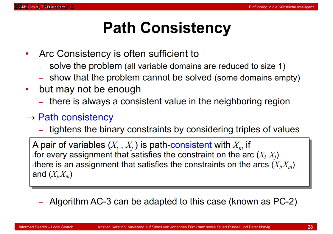
arcs()是超弧一致性。
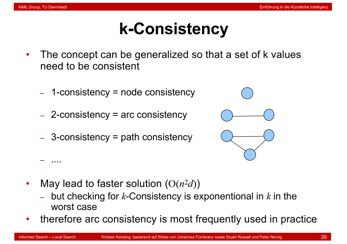
4.16 k-Consistency
4.17 Sudoku

255960怎么来的??
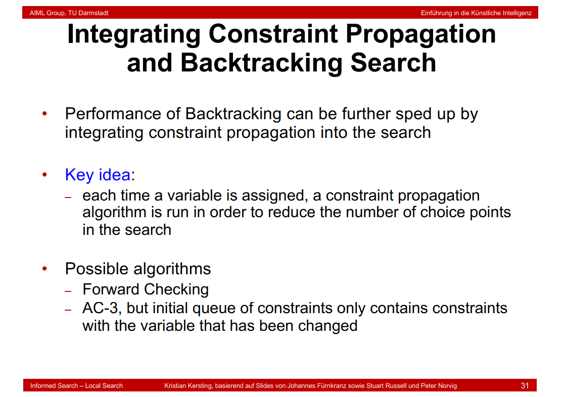
4.18 Integrating Constraint Propagation and Backtracking Search
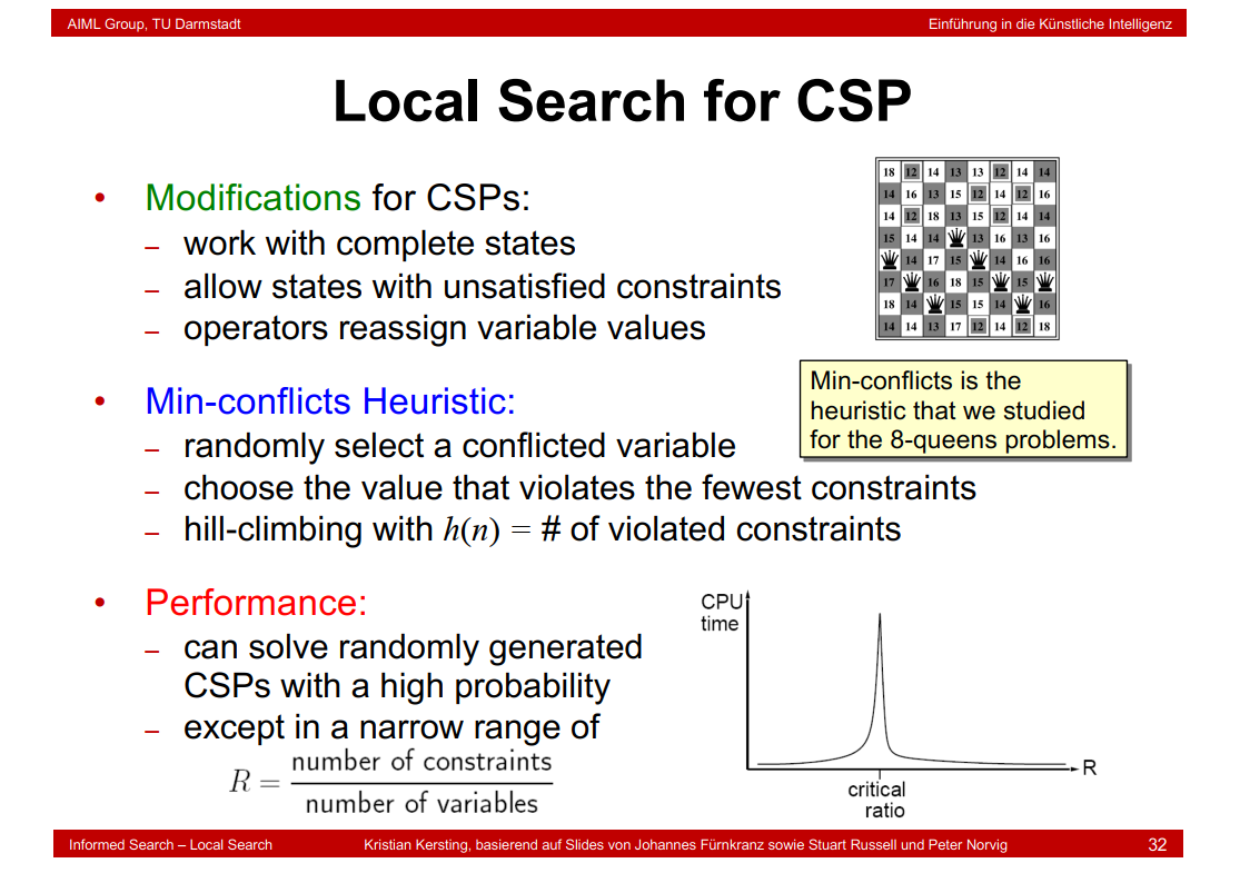
4.19 Local Search for CSP
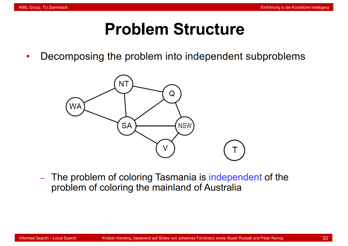
4.20 Problem Structure
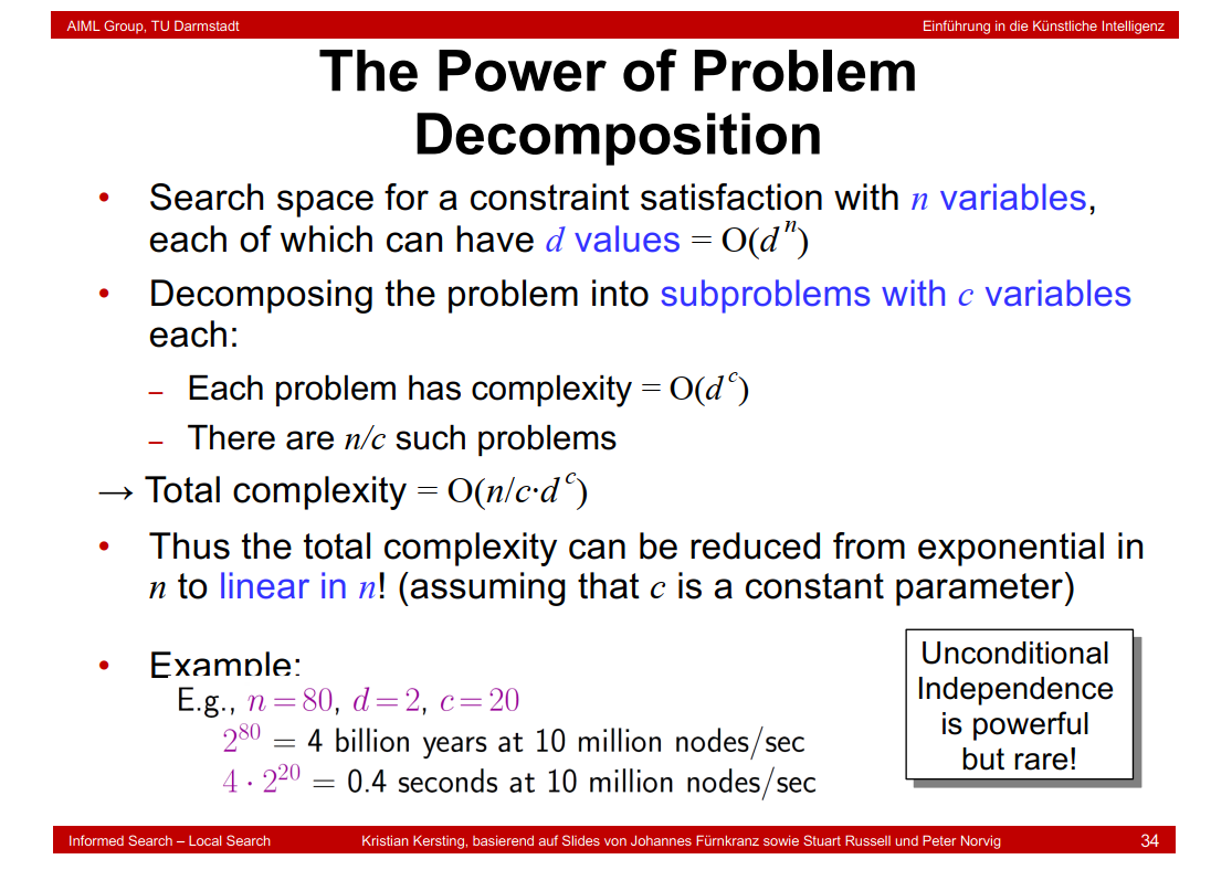
4.21 The Power of Problem Decomposition
4.22 Tree-Structured CSP
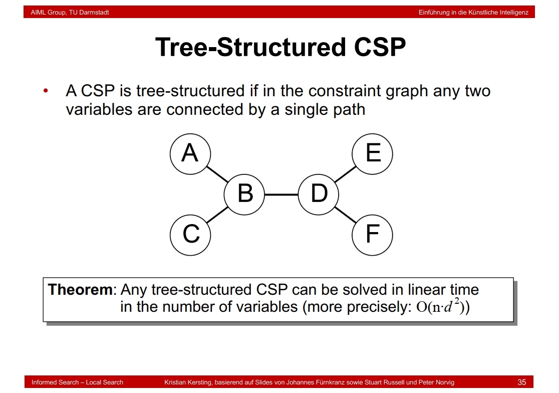
为什么是O(n\(d^2\))
4.23 Linear Algorithm for Tree-Structured CSPs

4.24 Nearly Tree-structured Problems
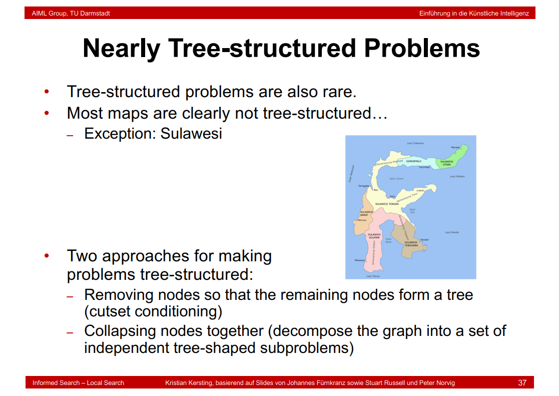
4.25 Cutset Conditioning

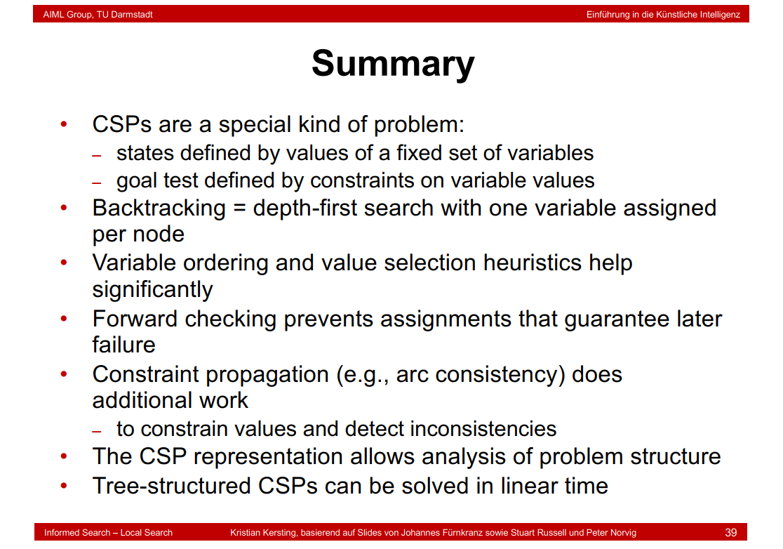
4.26 Summary
5.logic
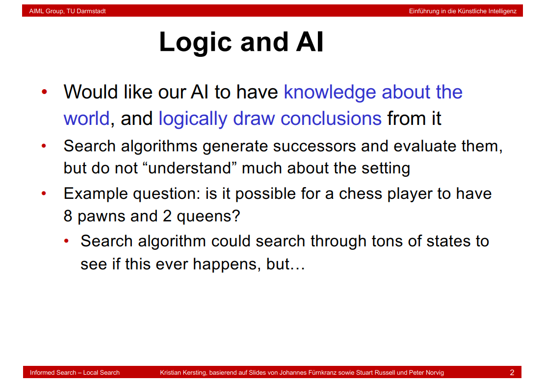
5.1 Logic and AI
5.2 Exploring a wumpus world
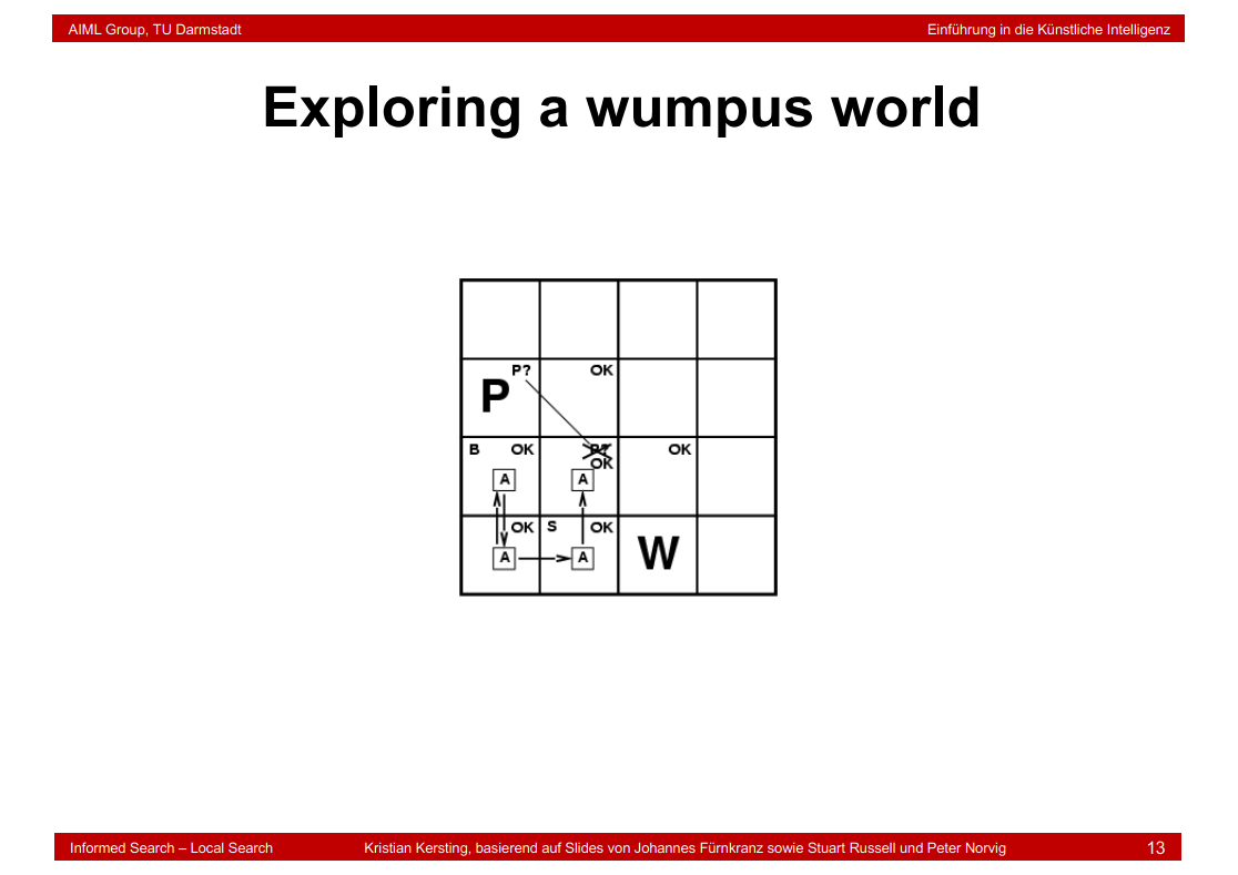
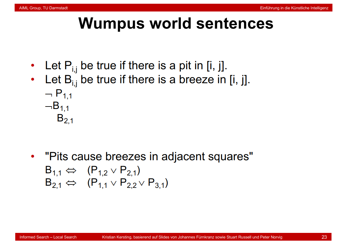
P是pit,B是Breeze
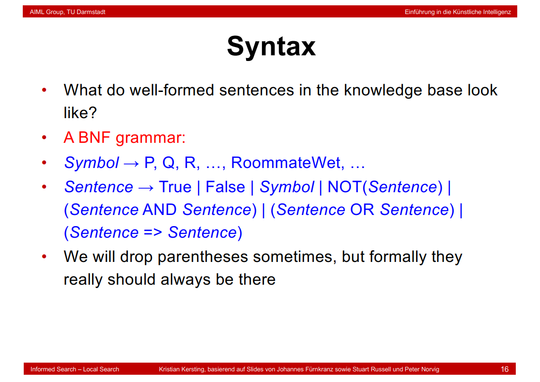
5.3 Syntax
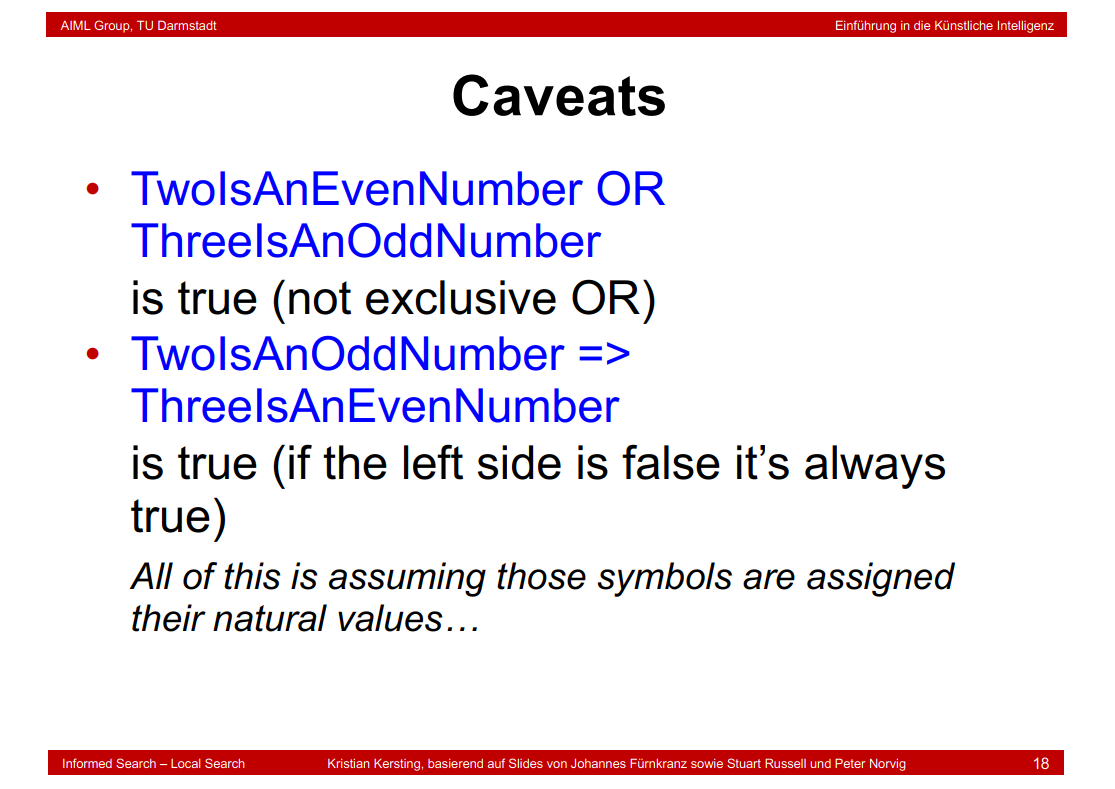
5.4 Caveats
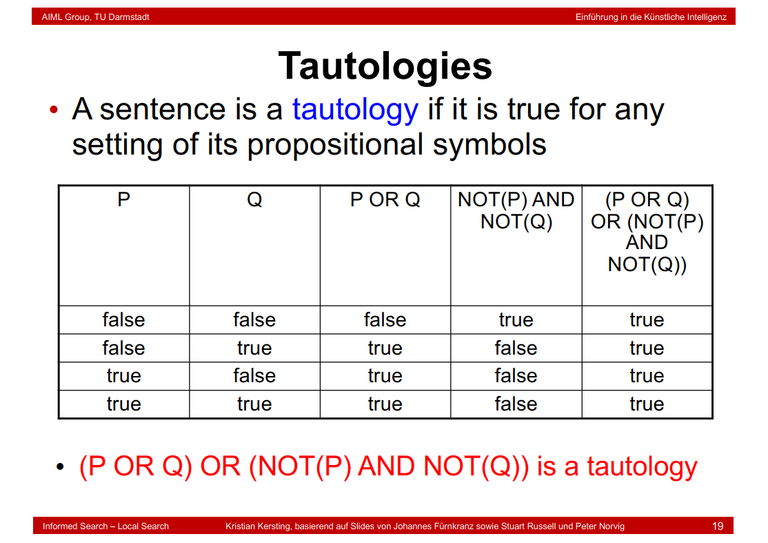
5.5 Tautologies
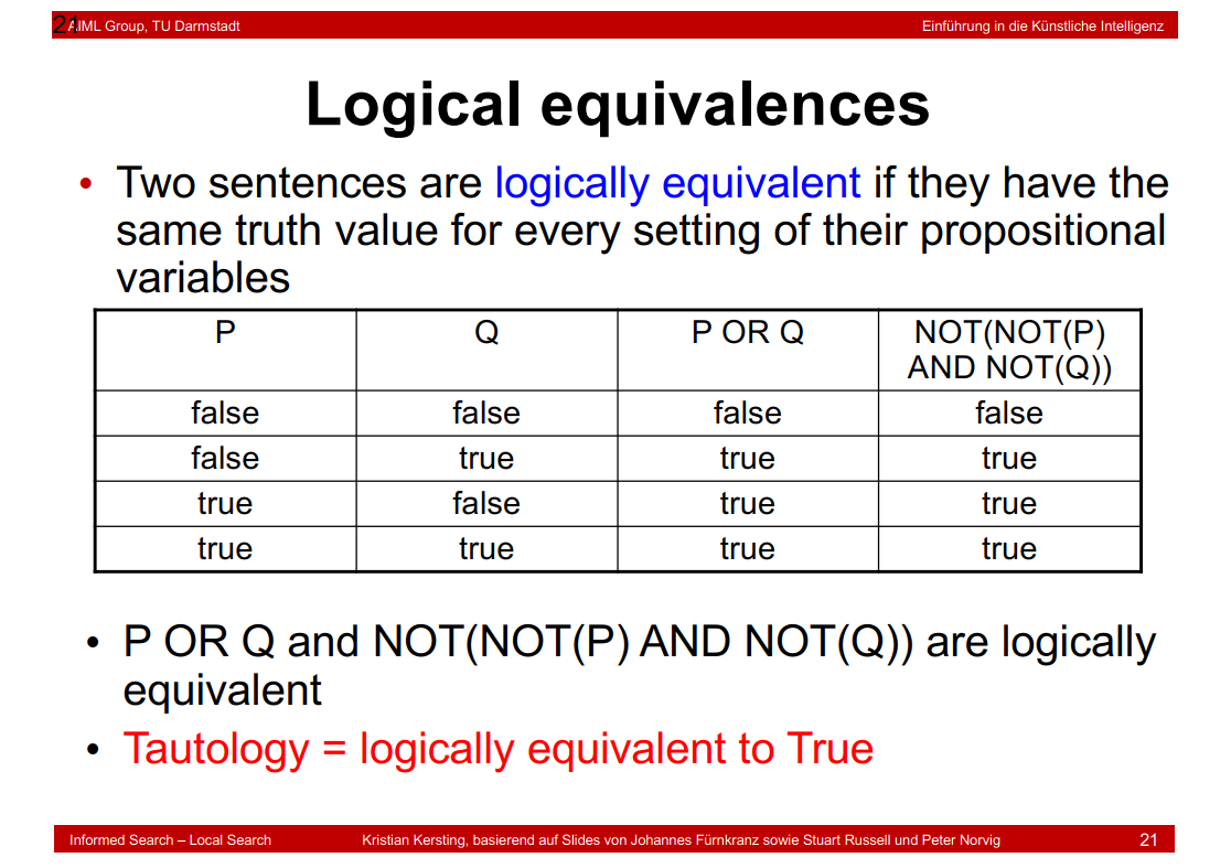
5.6 Logical equivalences
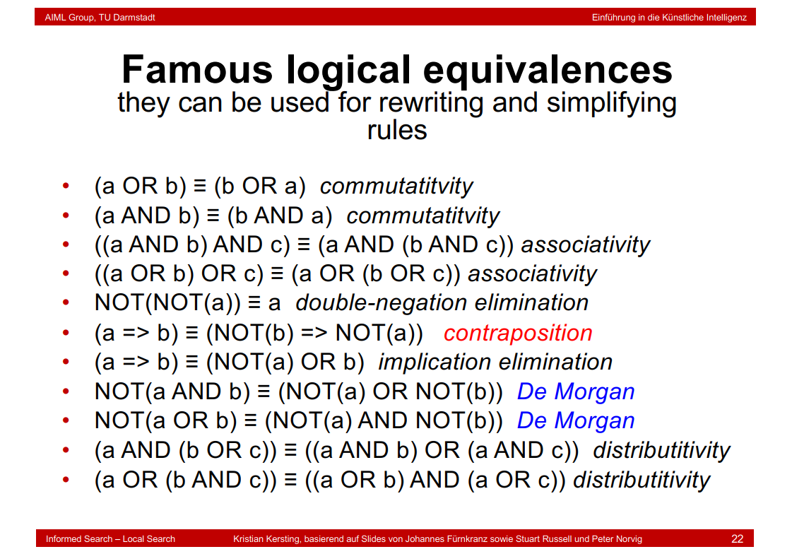
5.7 Famous logical equivalences
5.8 Wumpus world sentences
5.9 Inference

5.10 Wumpus Truth tables for inference
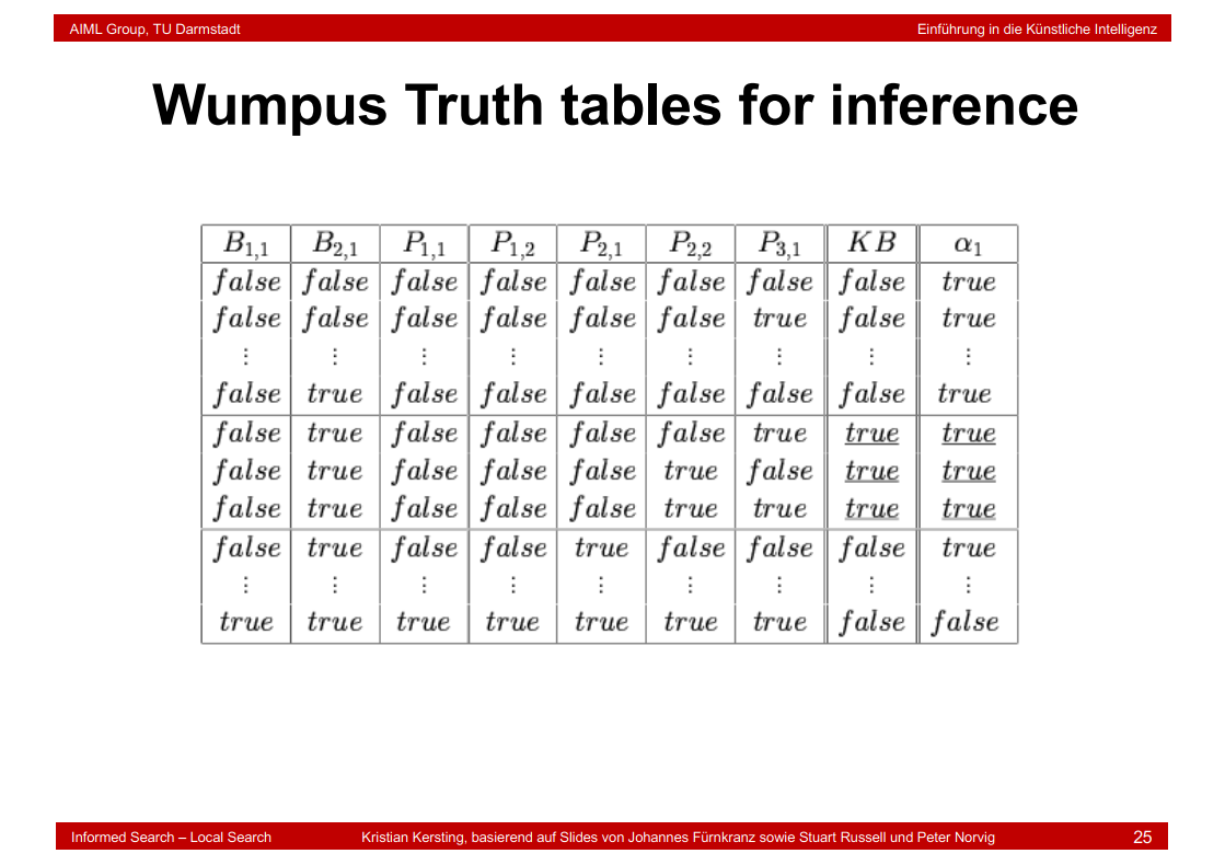
we assume that all formulas in our knowledge base are true.
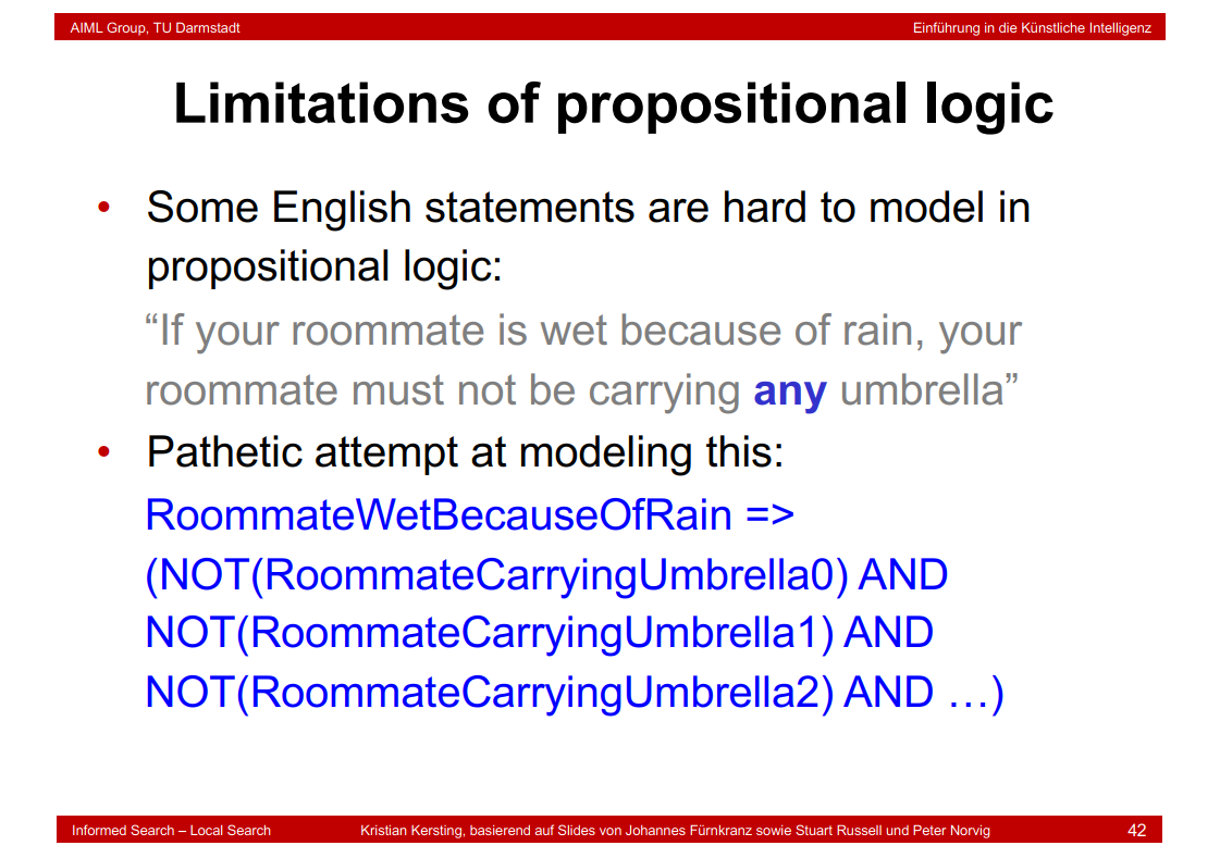
5.11 Limitations of propositional logic
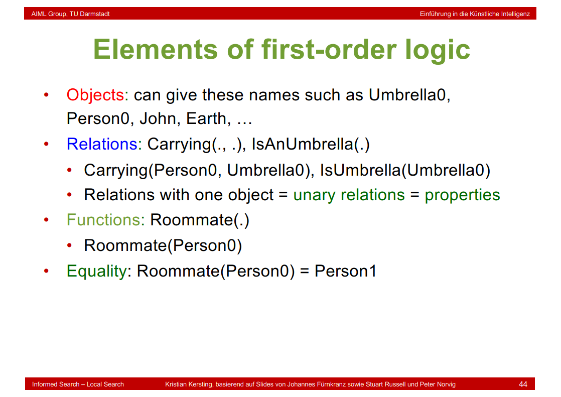
5.12 Elements of first-order logic
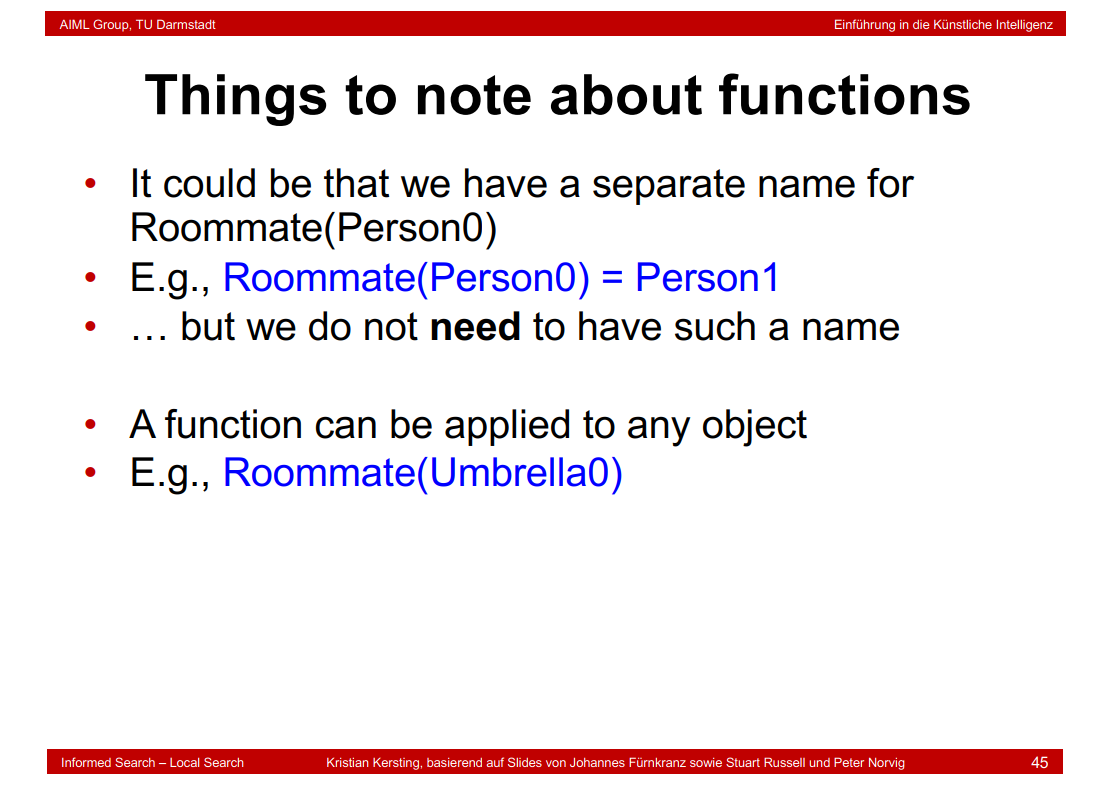
5.13 Things to note about functions
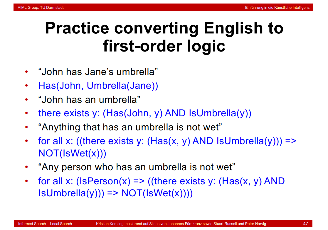
5.14 Practice converting English to first-order logic
5.15 More practice converting English to first-order logic

5.16 Even more practice converting English to first-order logic…

5.17 More realistically…

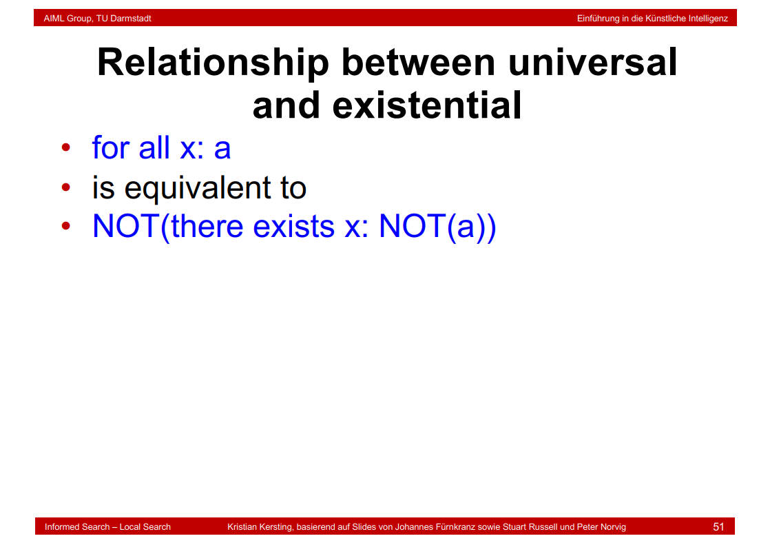
5.18 Relationship between universal and existential
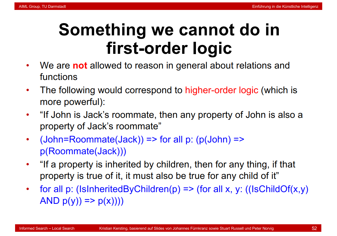
5.19 Something we cannot do in first-order logic
5.20 Axioms and theorems
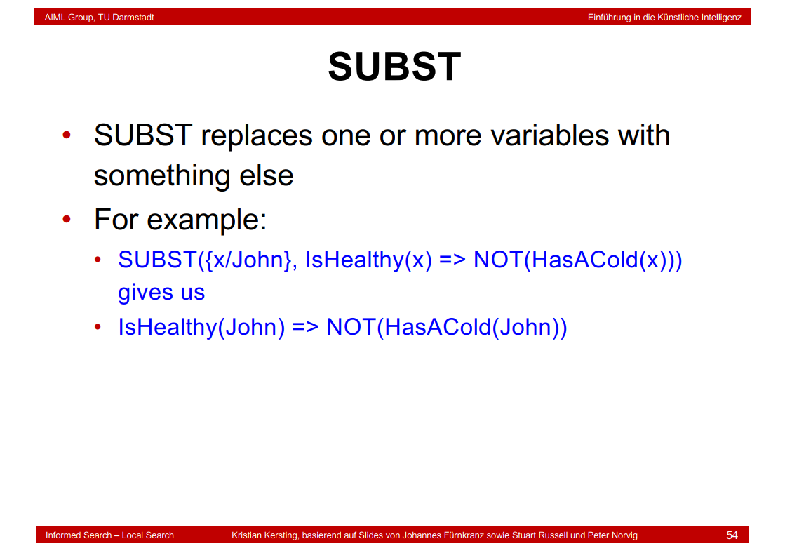
5.21 SUBST
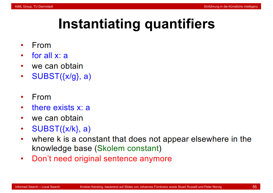
5.22 Instantiating quantifiers
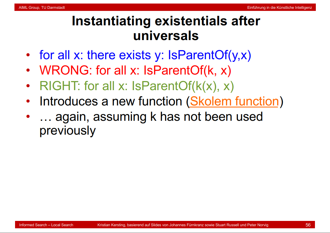
5.23 Instantiating existentials after universals
5.24 Generalized modus ponens

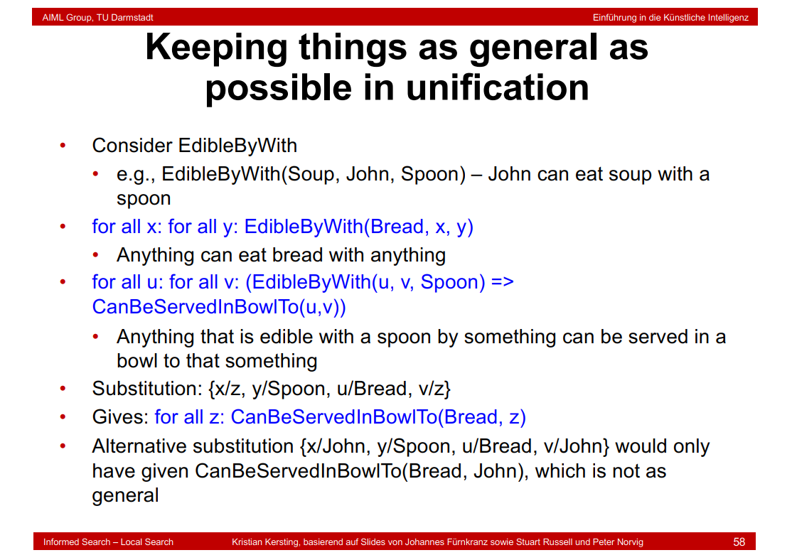
5.25 Keeping things as general as possible in unification
5.26 Resolution for first-order logic
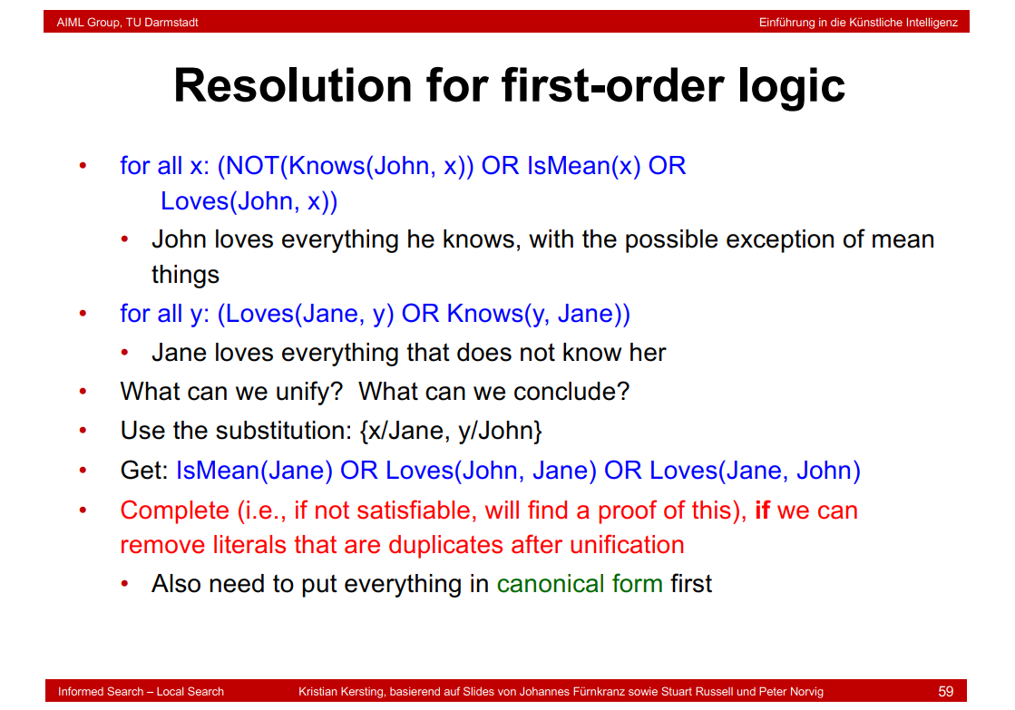
for all y: (Loves(Jane, y) OR Knows(y, Jane))
Jane loves everything that does not know her
这里用xor更佳。
5.27 Special case: Horn clauses(补充)
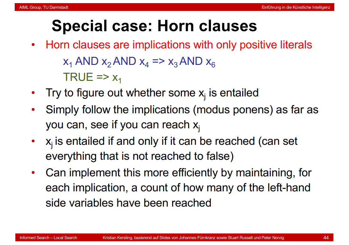
Horn clauses也可以写成两句话的形式,结果和课件一致。
x1AND x2 AND x4=> x3
x1AND x2 AND x4=> x6
Beachte auch, dass, wenn man die Formel auf der Folie auflöst, man nicht eine Disjunktion mit zwei positiven Literalen bekommt, sondern eine Konjunktion von zwei Horn Klauseln:
NOT x1 OR NOT x2 OR NOT x4 OR (x3 AND x6)
= (NOT x1 OR NOT x2 OR NOT x4 OR x3) AND (NOT x1 OR NOT x2 OR NOT x4 OR x6).
6. Planning
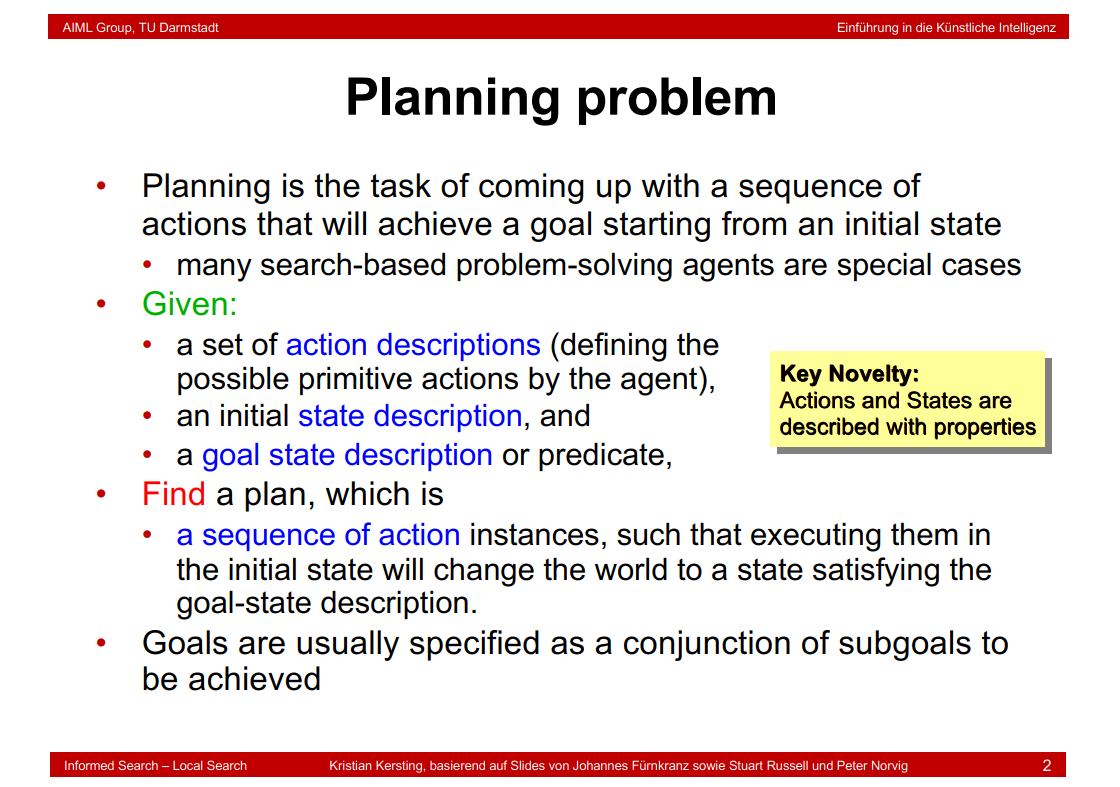
6.1 Planning Problem
6.2 Application Scenario
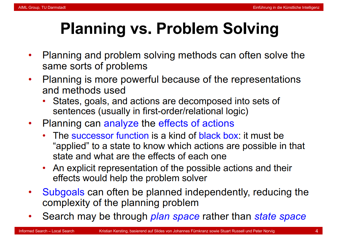
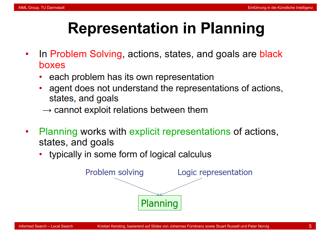
6.3 Planning vs. Problem Solving
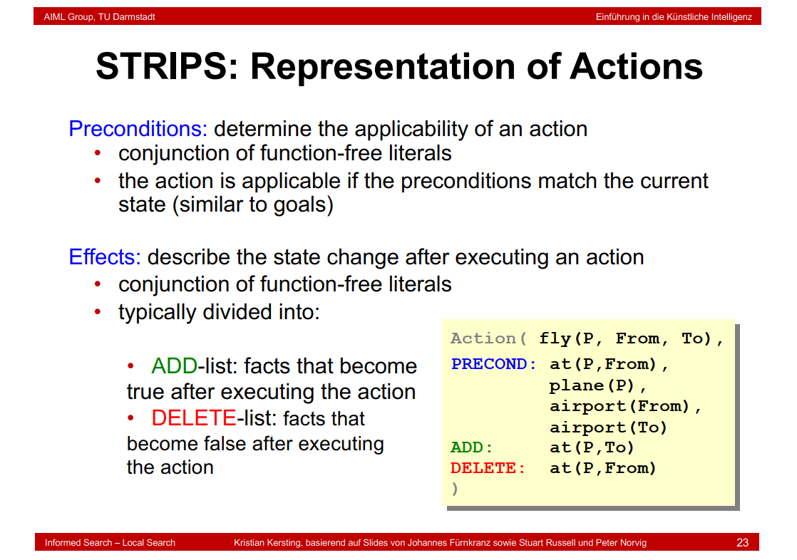
6.4 Representation in Planning
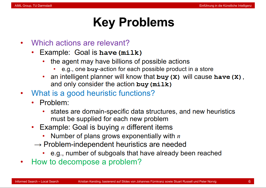
6.5 Key Problems
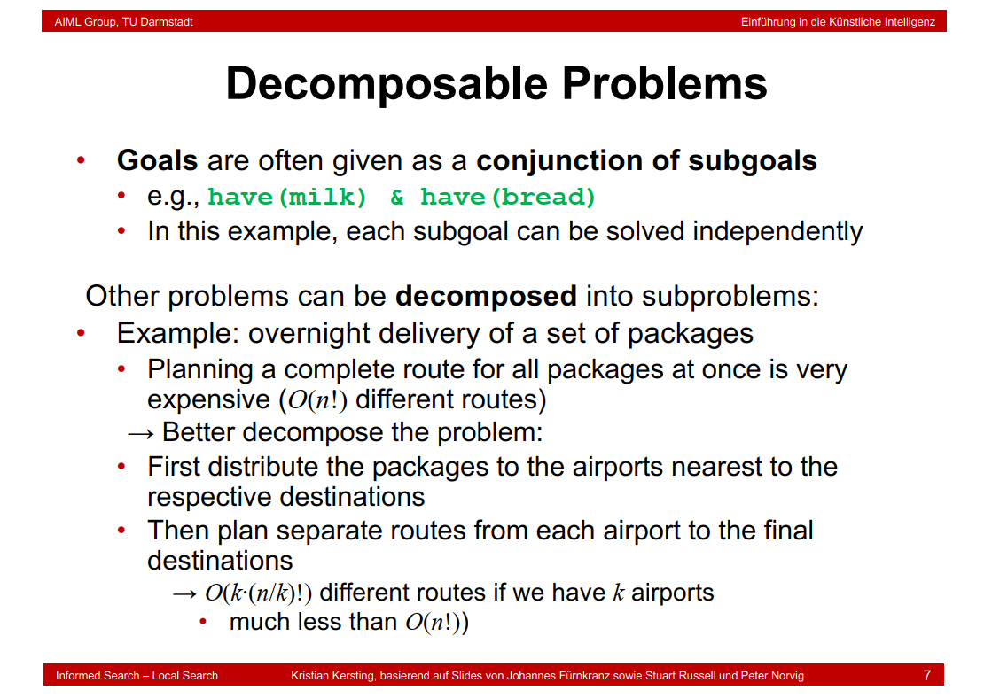
6.6 Decomposable Problems
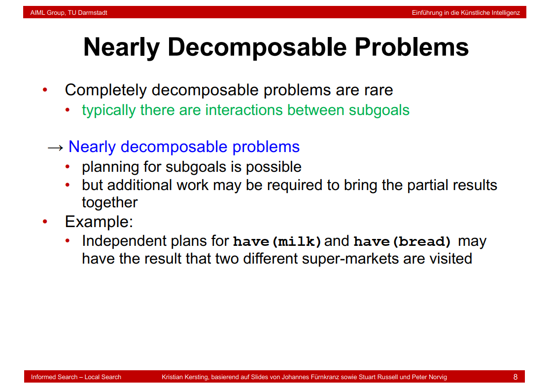
6.7 Nearly Decomposable Problems
6.8 Planning in First-Order Logic

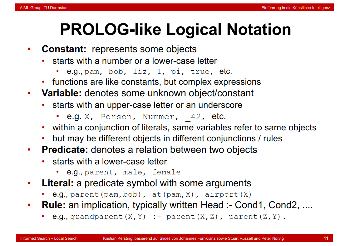
6.9 PROLOG-like Logical Notation
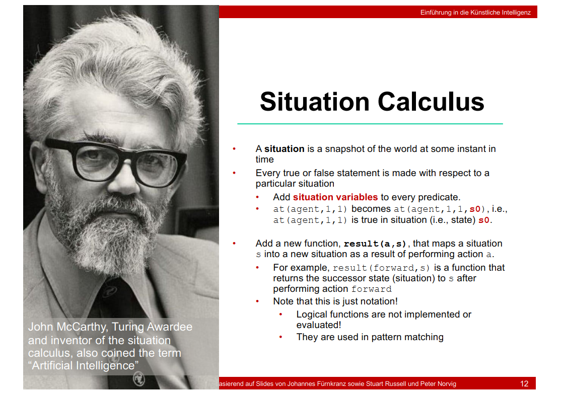
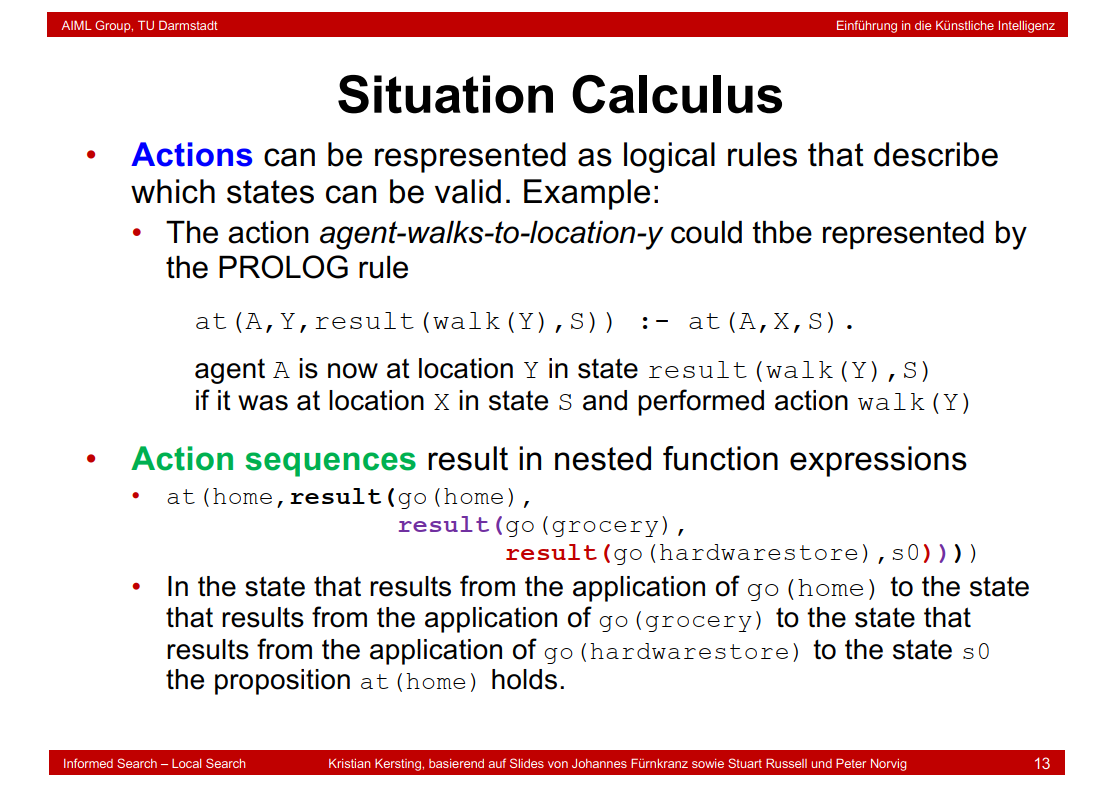
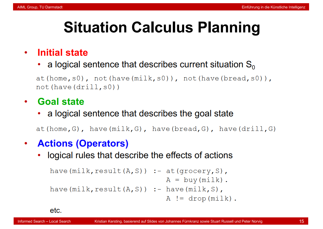
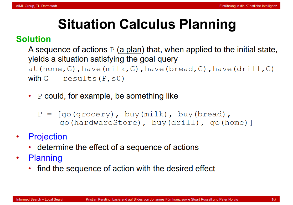
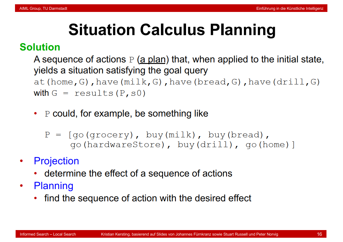
6.10 Situation Calculus
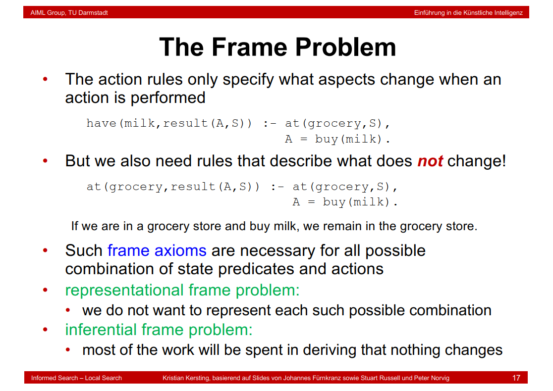
6.11 The Frame Problem
6.12 SC Planning: More Problems

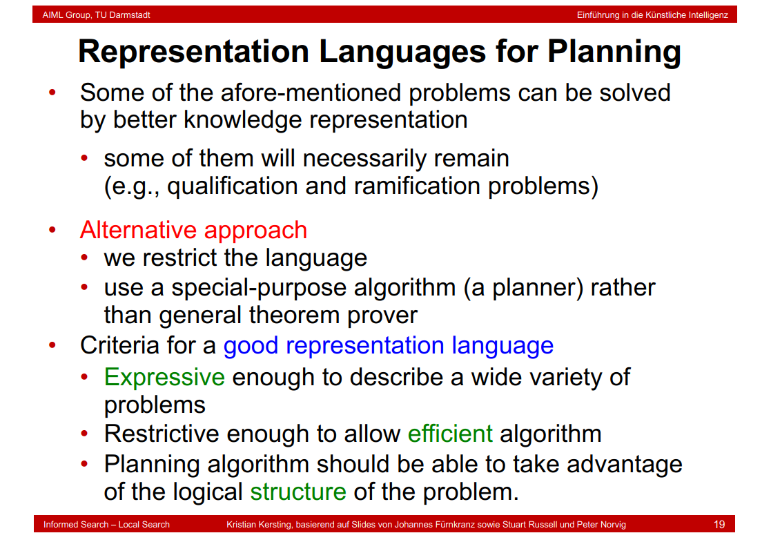
6.13 Representation Languages for Planning
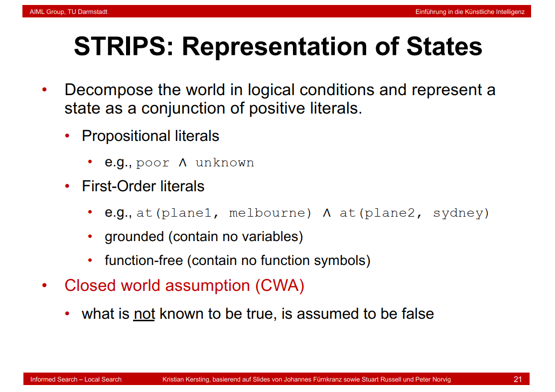
6.14 STRIPS: Representation of States
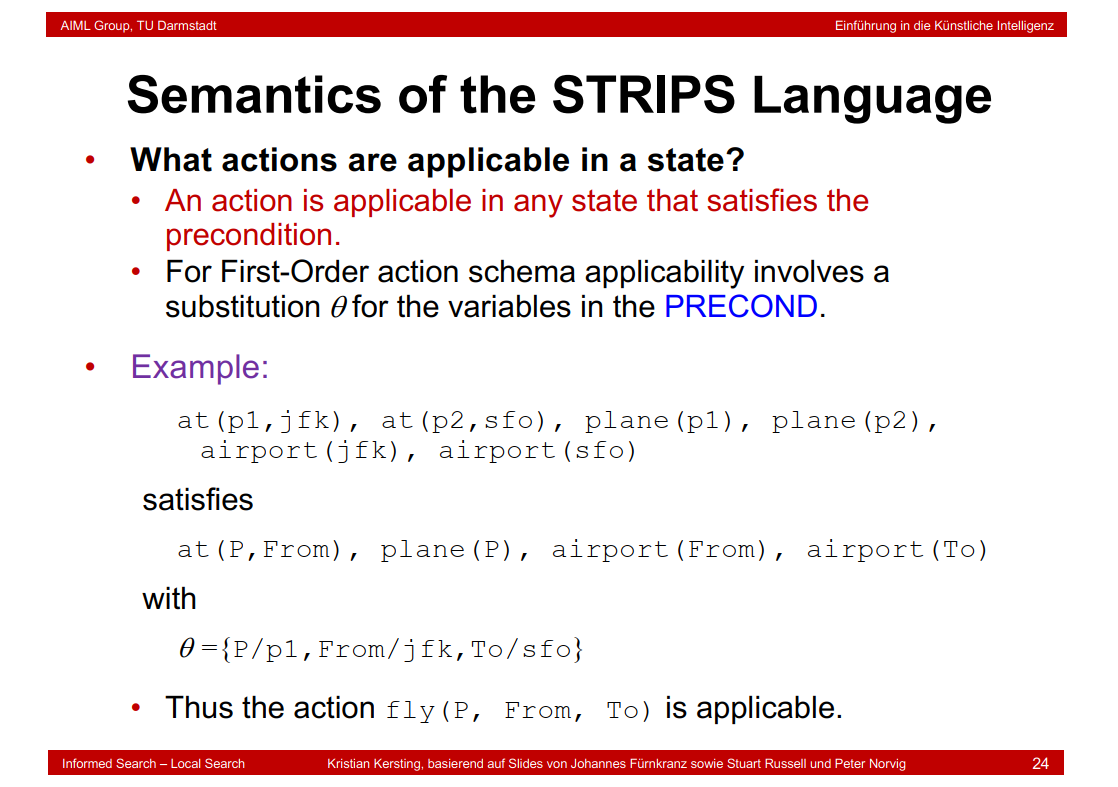
6.15 Semantics of the STRIPS Language
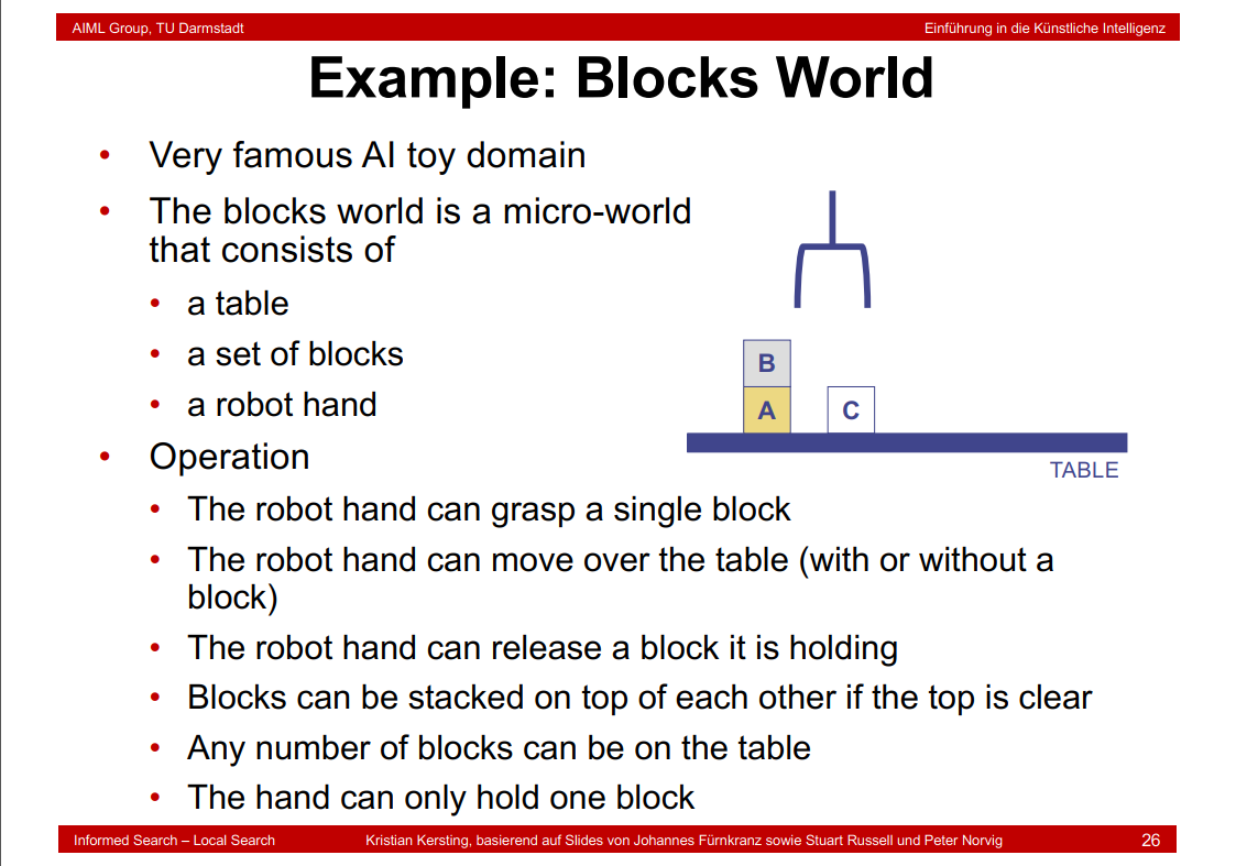
6.16 Example: Blocks World
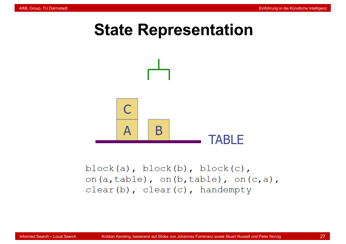
6.17 State Representation
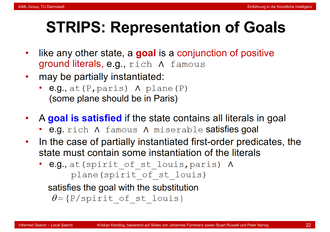
6.18 Goal Representation

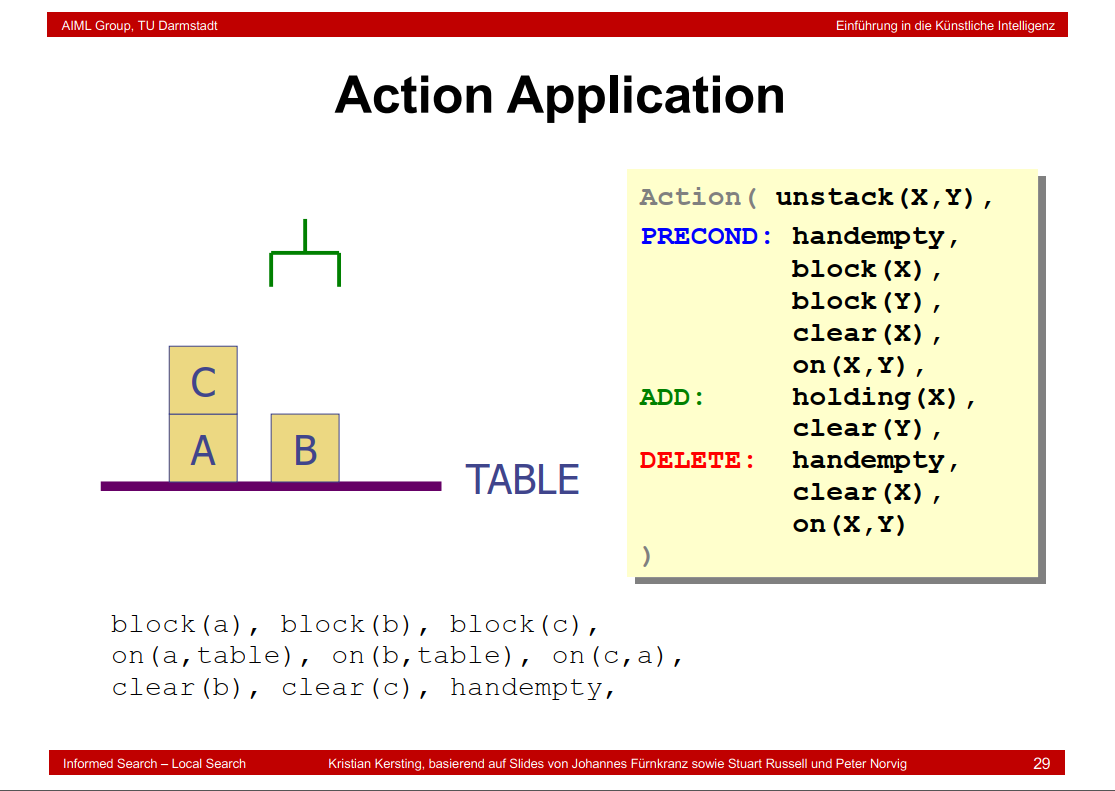
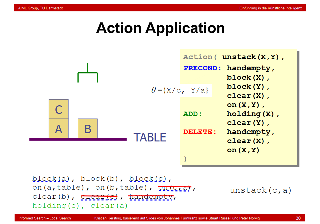
6.19 Action Application
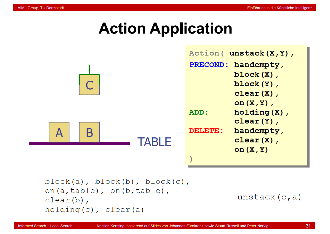
6.20 More Blocks-World Actions

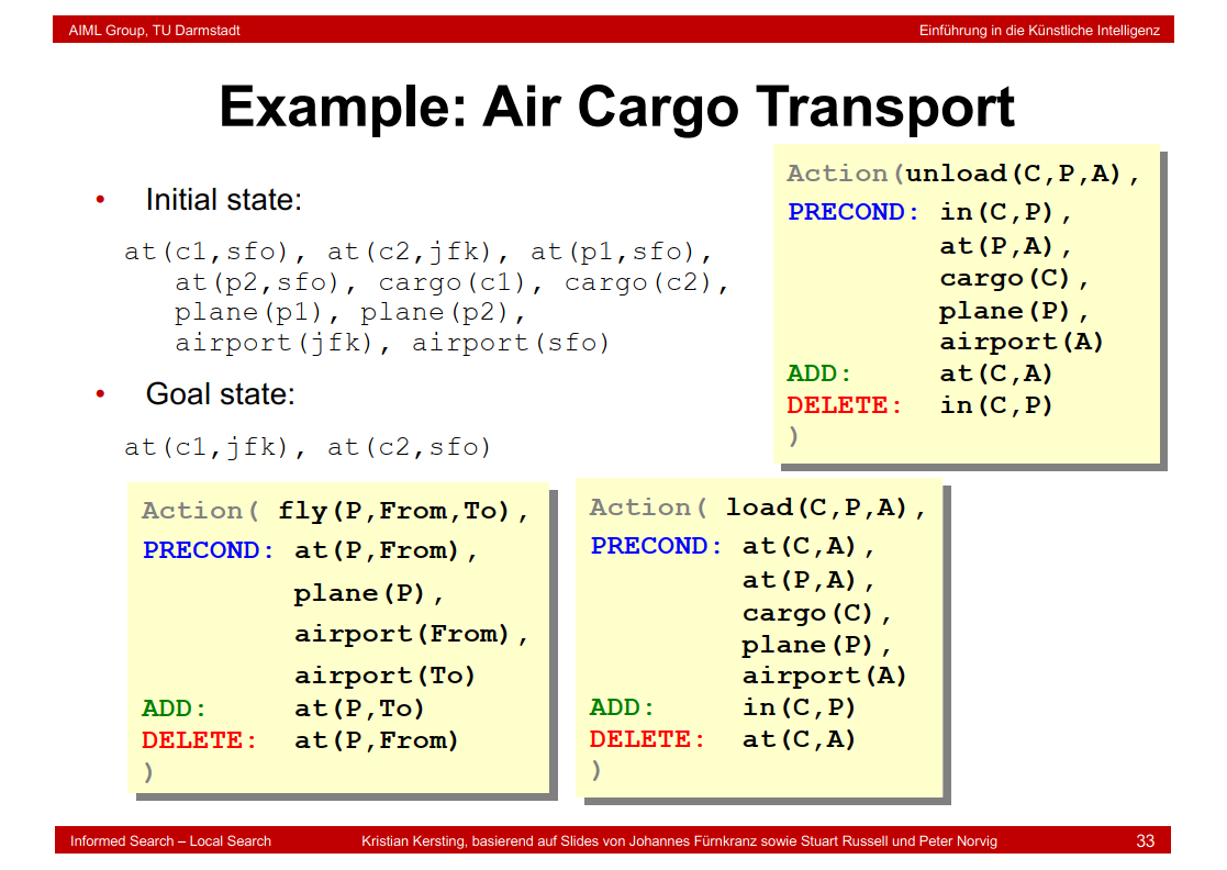
6.21 Example: Air Cargo Transport
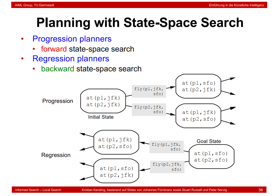
6.22 Planning with State-Space Search
6.23 Progression Algorithm

6.24 Regression Algorithm
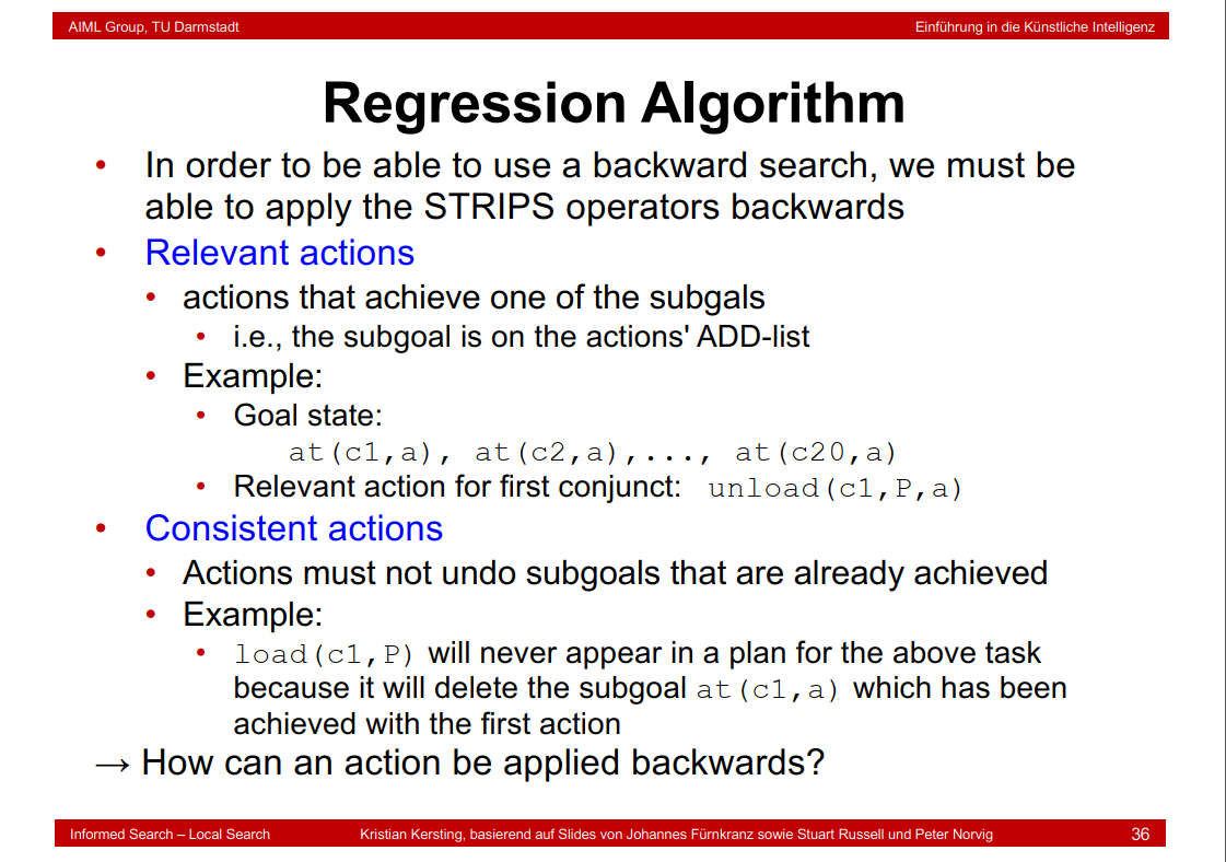
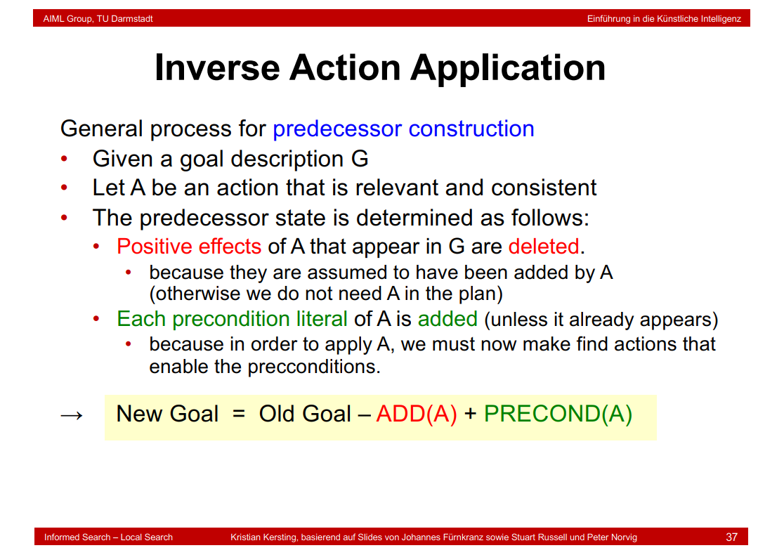
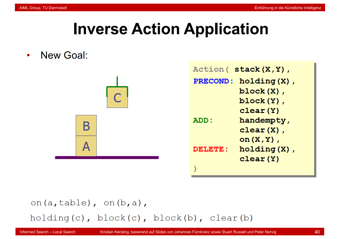
6.25 Inverse Action Application


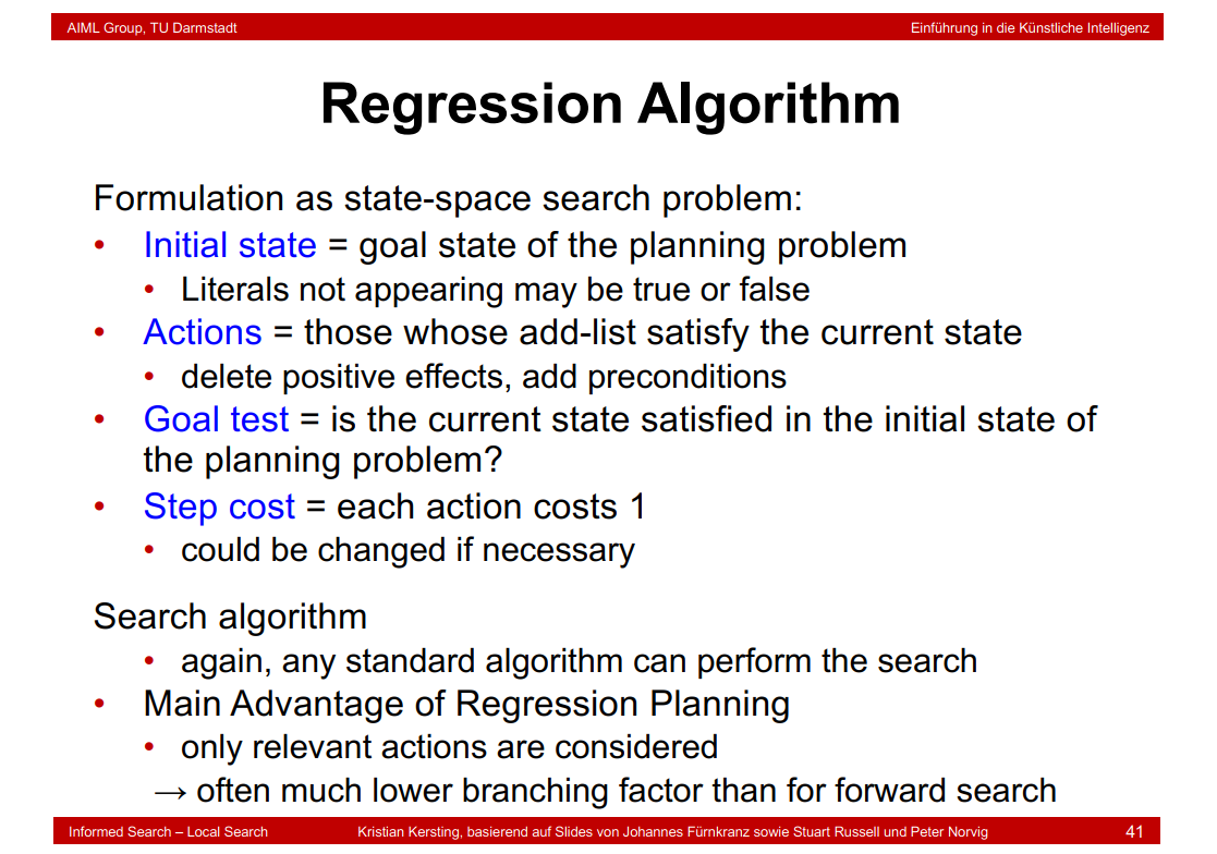
6.26 Regression Algorithm
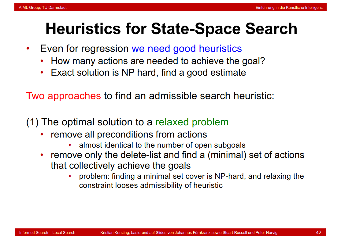
6.27 Heuristics for State-Space Search
6.28 Expressiveness and Extensions

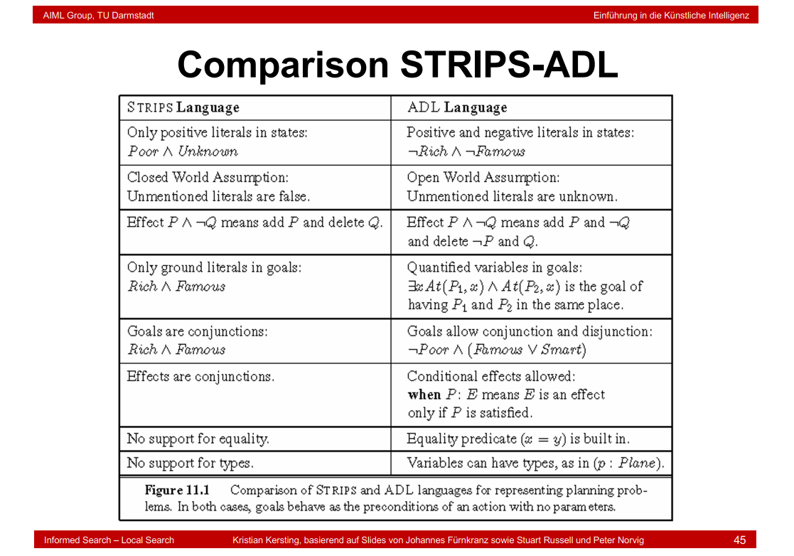
6.29 Comparison STRIPS-ADL
7. Deep learning
7.1 Learning
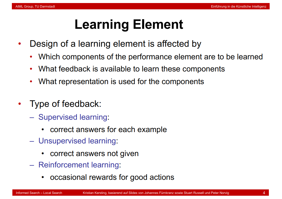
7.2 Learning Element
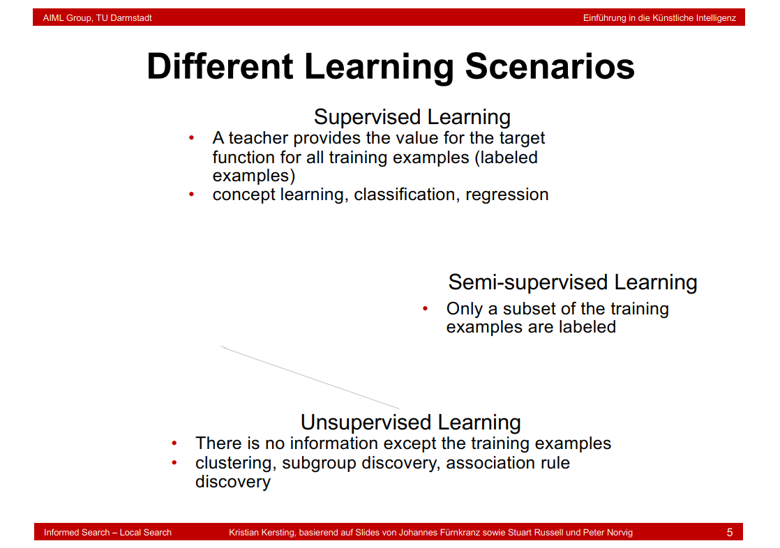
7.3 Different Learning Scenarios
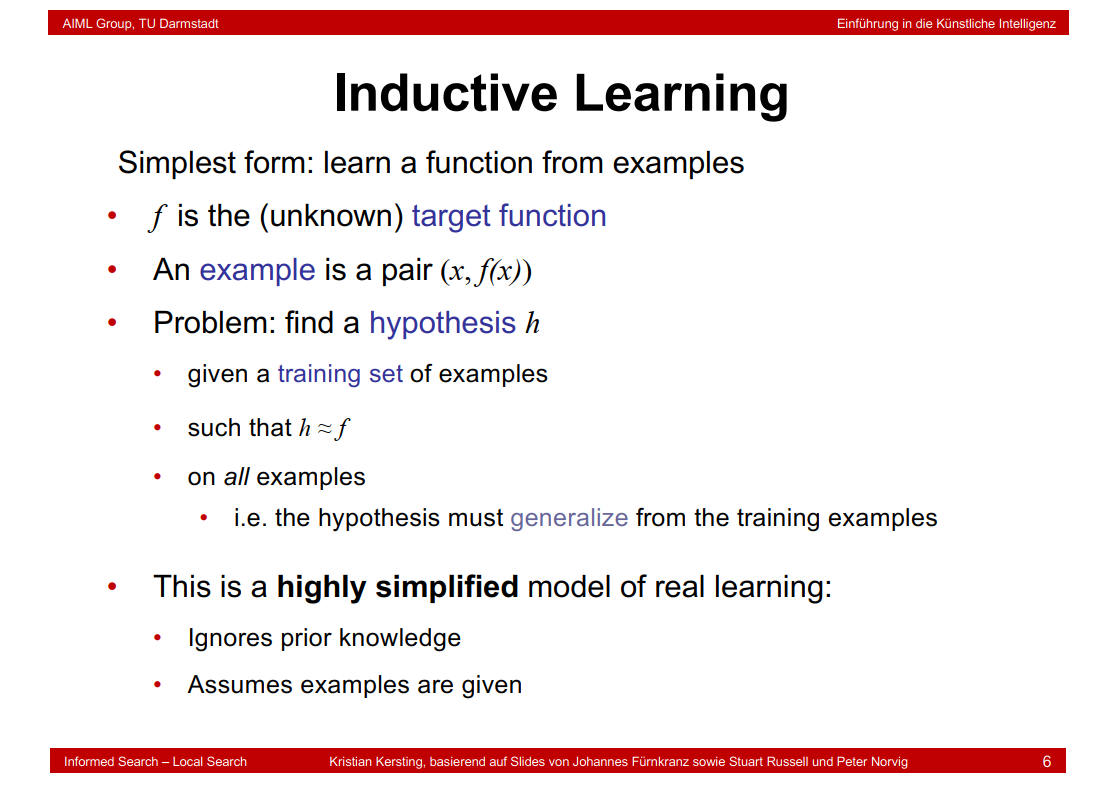
7.4 Inductive Learning
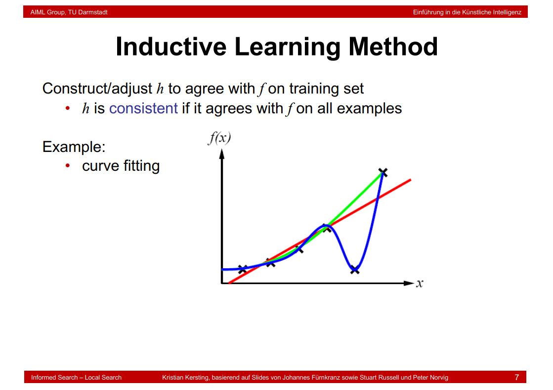
7.5 Inductive Learning Method

7.6 Performance Measurement

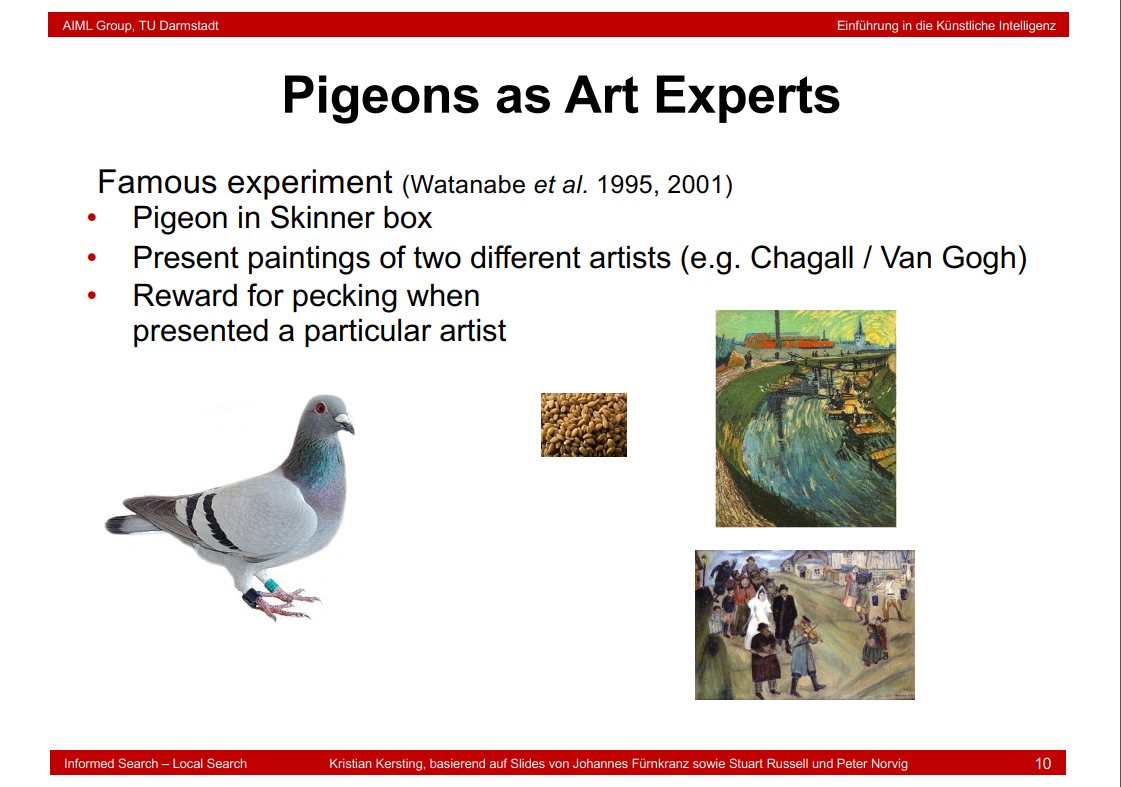
7.7 Pigeons as Art Experts
7.8 Results
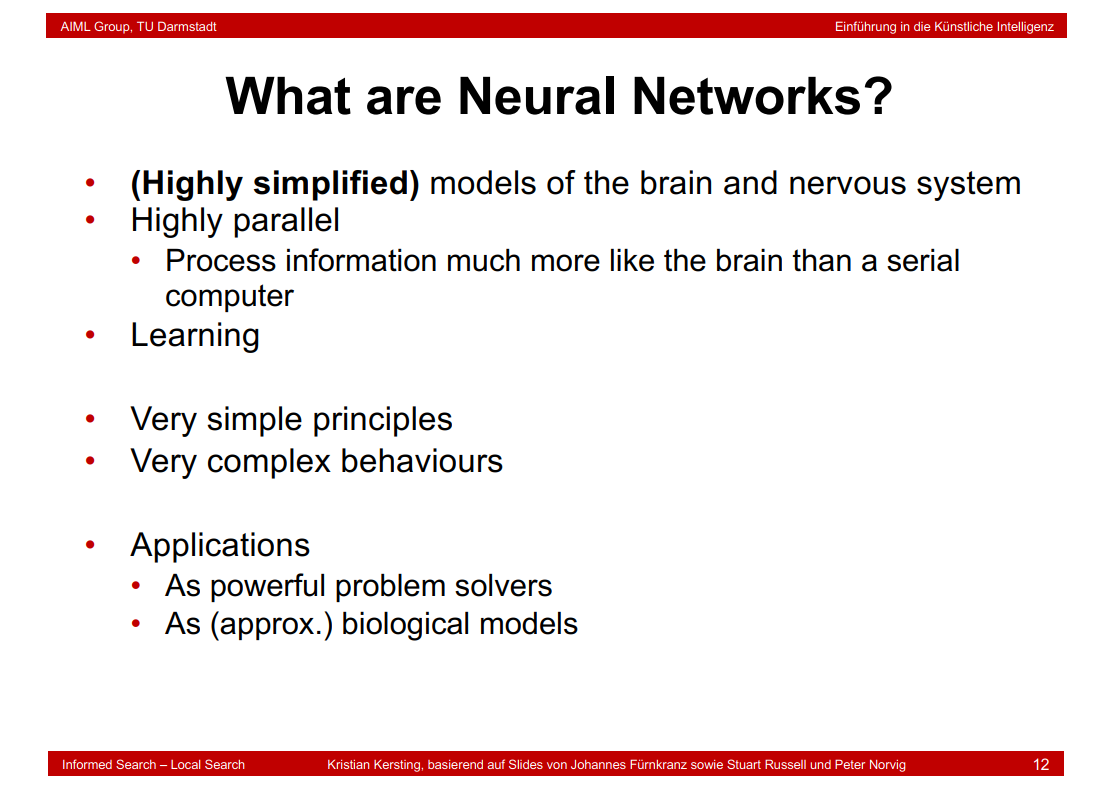
7.9 What are Neural Networks?
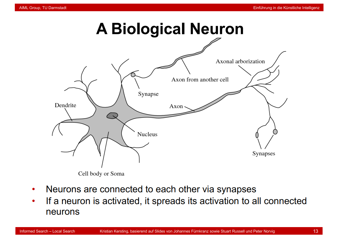
7.10 A Biological Neuron
7.11 An Artificial Neuron
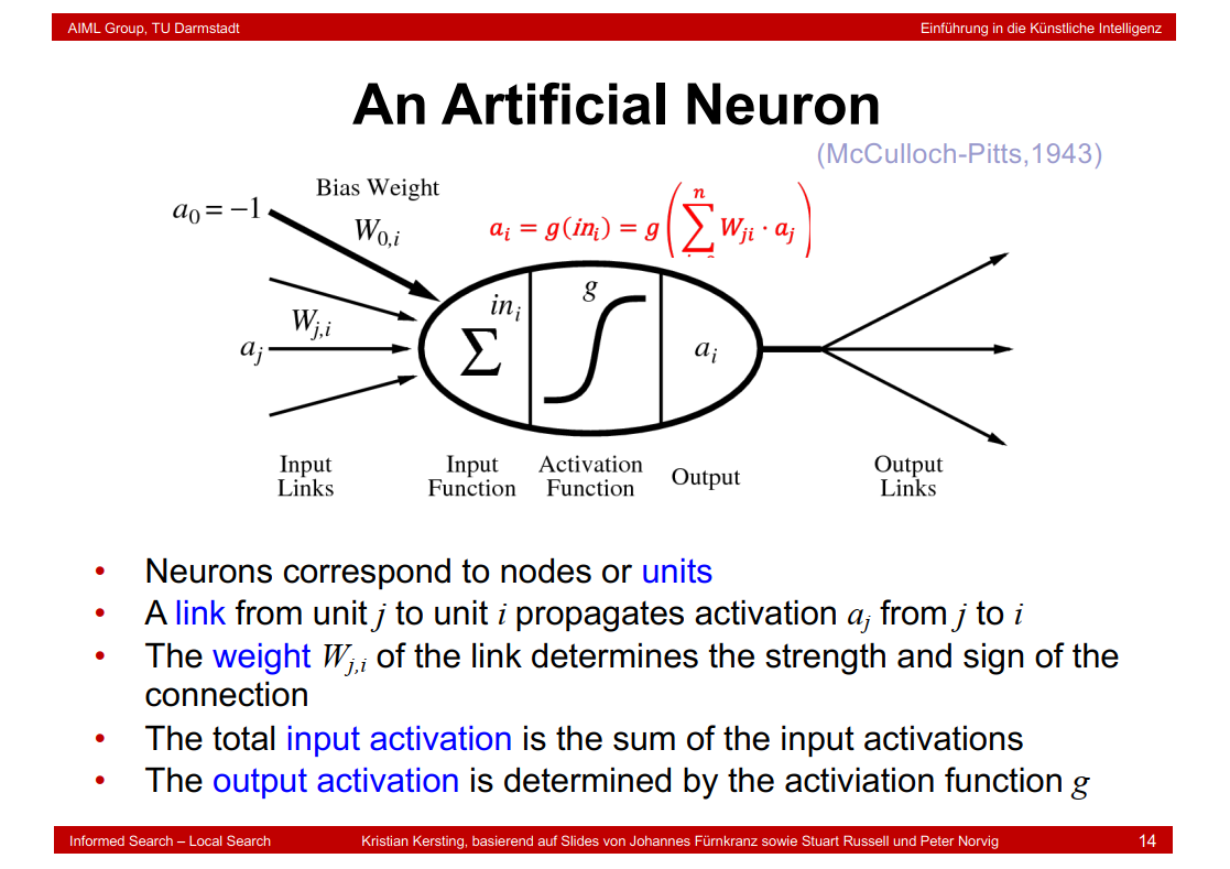
\(a_{j}\)是输出,\(a_{i}\)是输入;
\(W_{j,i}\)决定了连接的强度和sign;
g是激活函数。
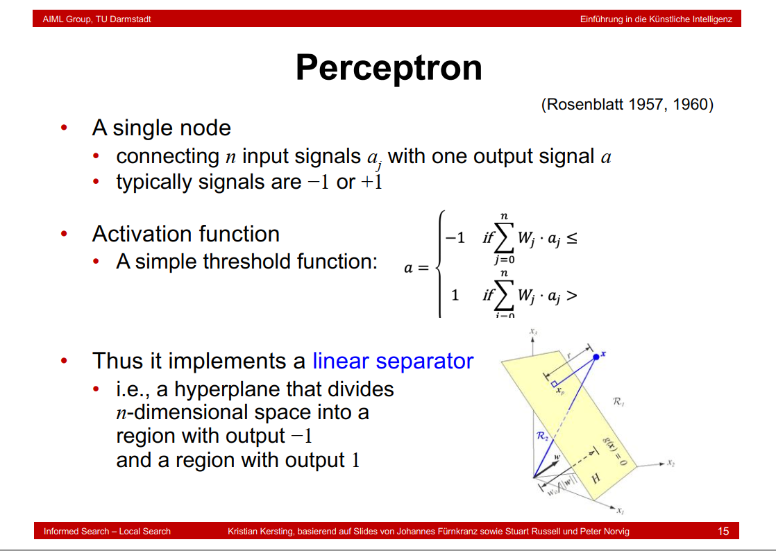
7.12 Perceptron
7.13 Perceptrons and Boolean Functions
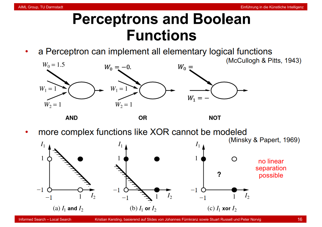
\(I_1\)和\(I_2\)表示两个待做运算的输入变量。这里想说明的是xor问题线性不可分。
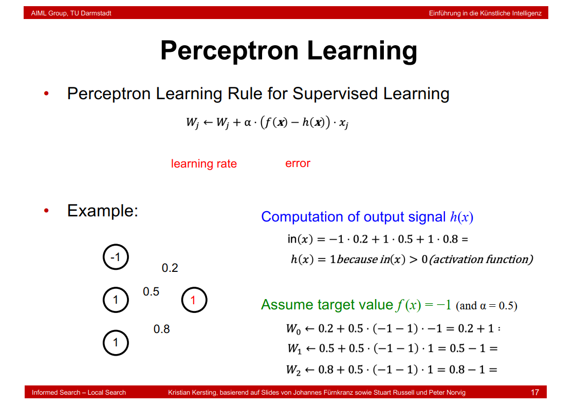
7.14 Perceptron Learning
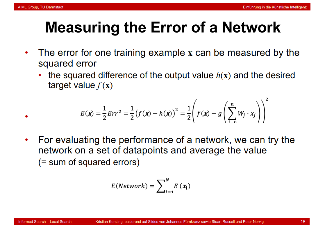
7.15 Measuring the Error of a Network
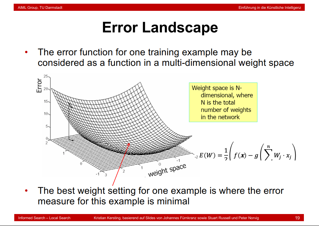
7.16 Error Landscape
7.17 Error Minimization via Gradient Descent
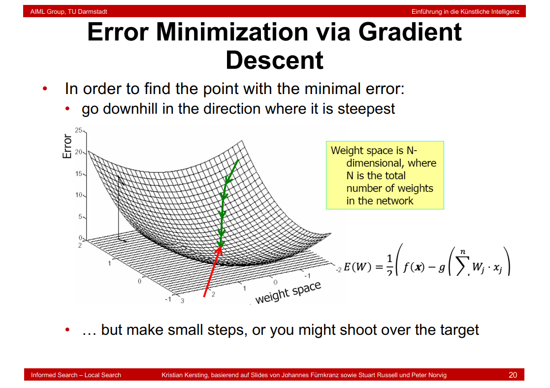
7.18 Error Minimization
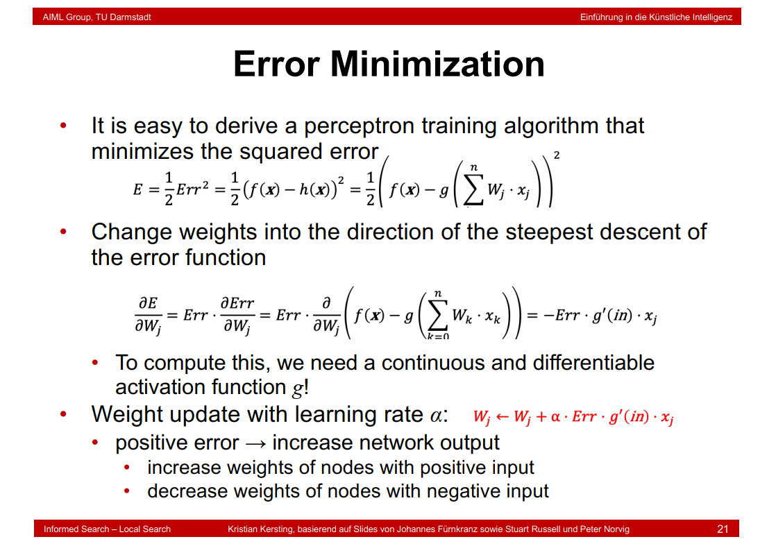
\(w_j\) \(\leftarrow\) \(w_j\) + \(\alpha\) * Err * g'(in) * \(x_j\) 和十七页的公式 \(w_j\) \(\leftarrow\) \(w_j\) + \(\alpha\) * (f(x) - h(x)) * \(x_j\) 不同的原因在于前者没有激活函数。
另一种形式是\(w_j\) \(\leftarrow\) \(w_j\) - \(\alpha\)*\(\frac{dL}{dw_j}\)
因为 \(\frac{dL}{dw_j}\) = g'(in) * \(x_j\) * \(\frac{dL}{dx_j}\)和 Err = -\(\frac{dL}{dw_j}\)
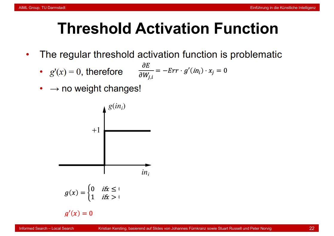
7.19 Threshold Activation Function
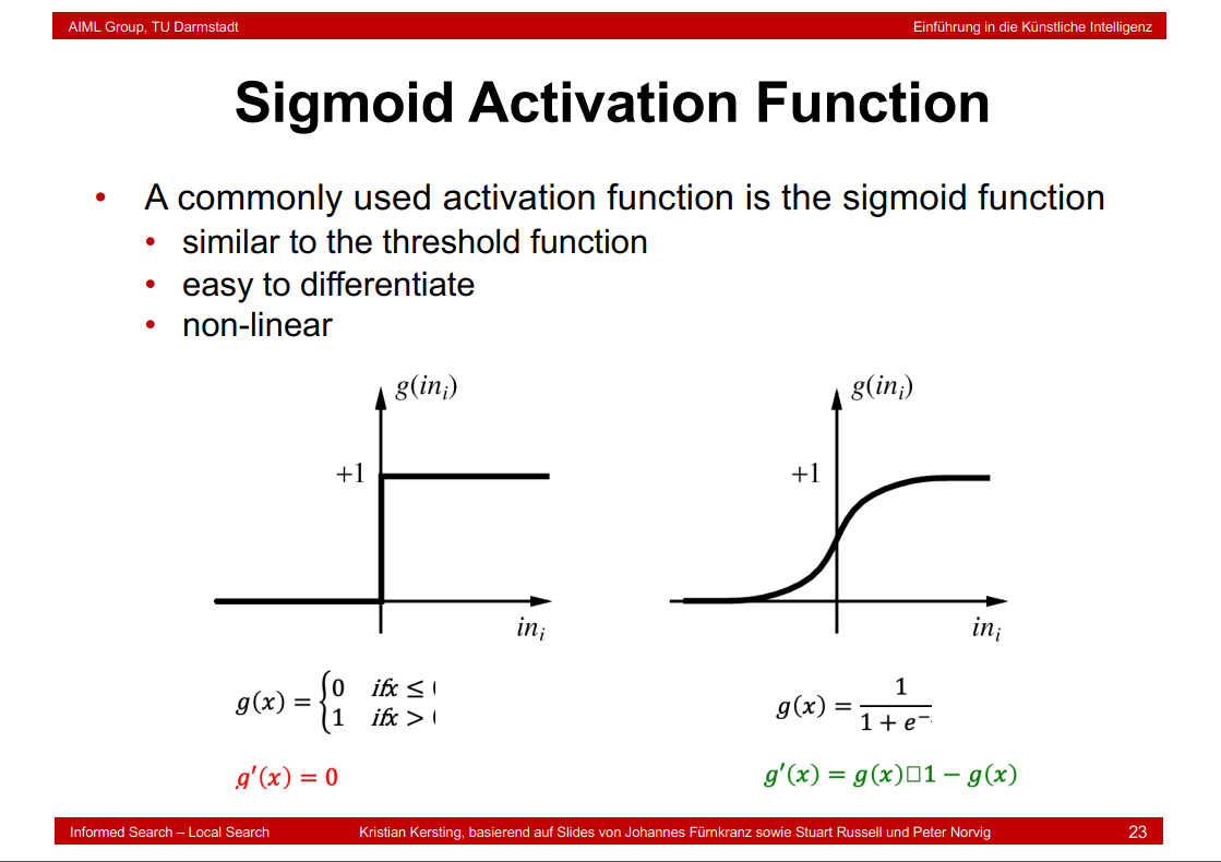
7.20 Sigmoid Activation Function
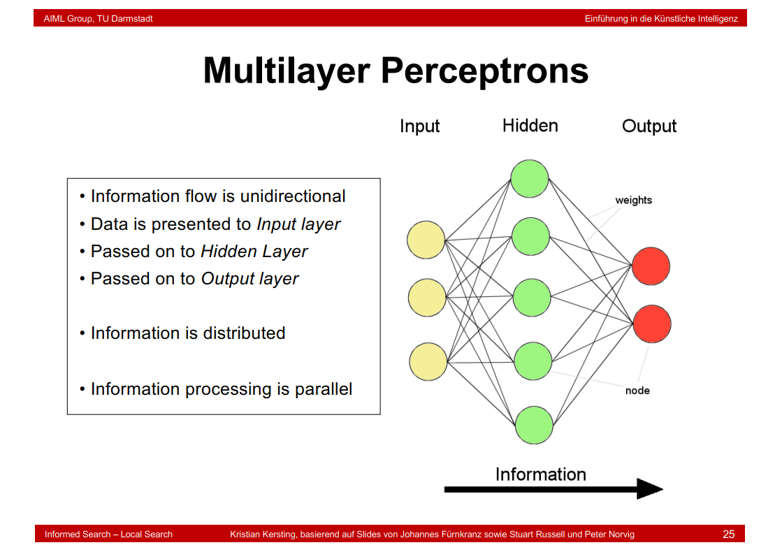
7.21 Multilayer Perceptrons
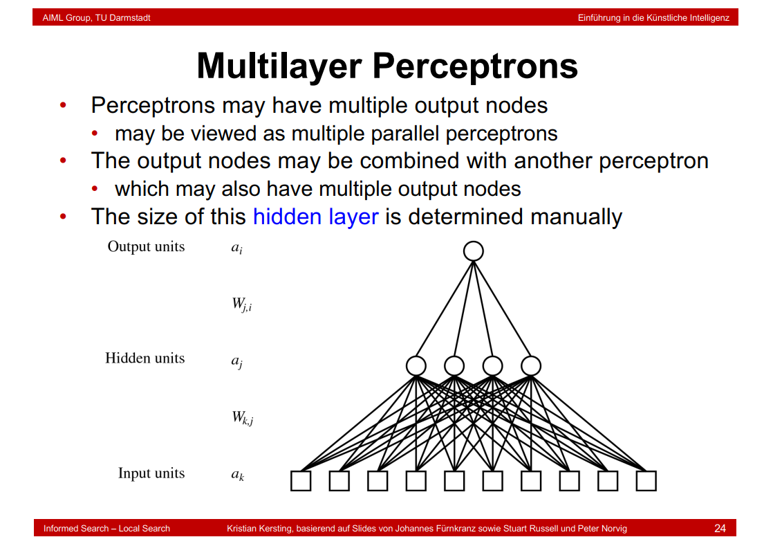
隐藏层表示训练数据不会提供关于网络的中间层会采用哪些值的信息,给人的感觉是"hidden"
7.22 Expressiveness of MLPs
7.23 Backpropagation Learning

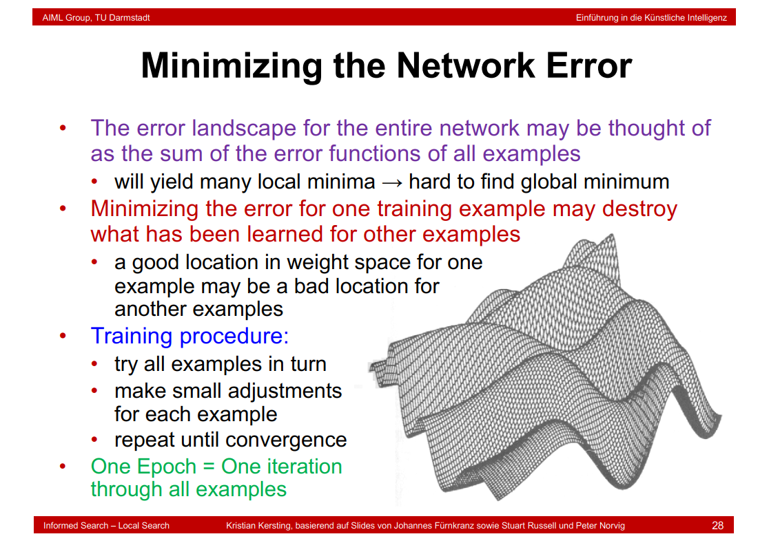
7.24 Minimizing the Network Error
7.25 Overfitting
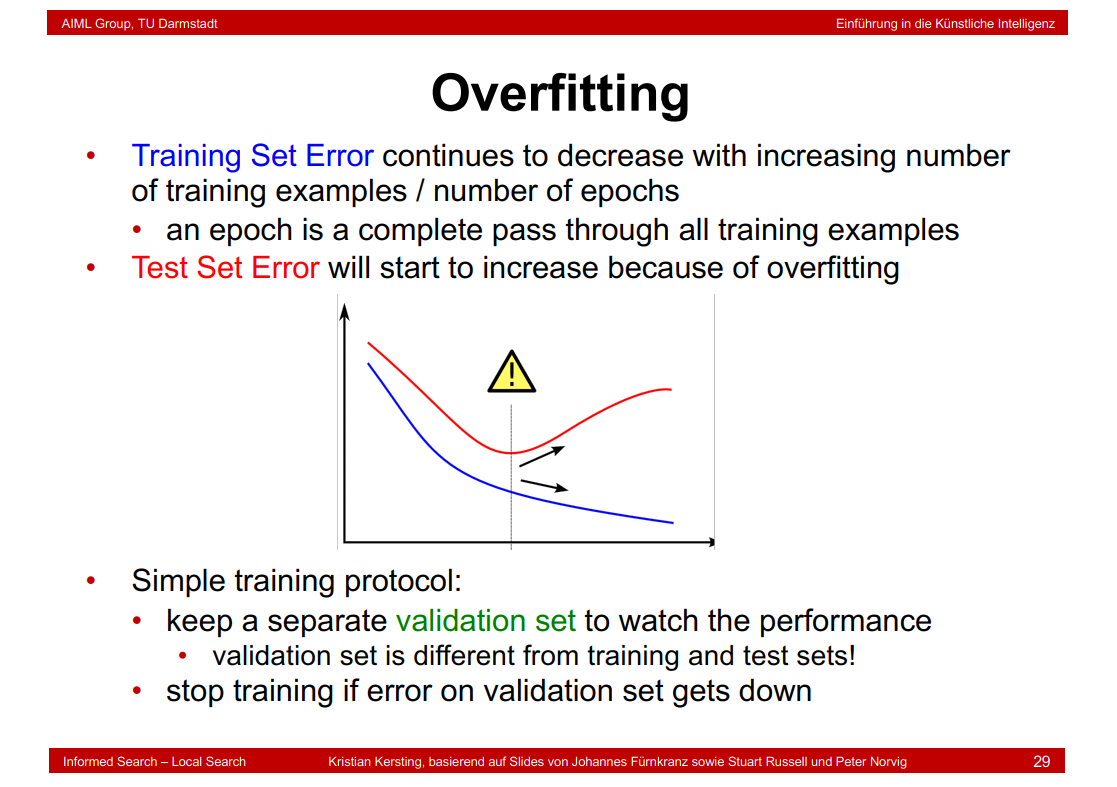
模型训练到红色曲线为最小值以防止过拟合。
7.26 Deep Learning
7.27 Goal of Deep Architectures

7.28 Deep Architectures

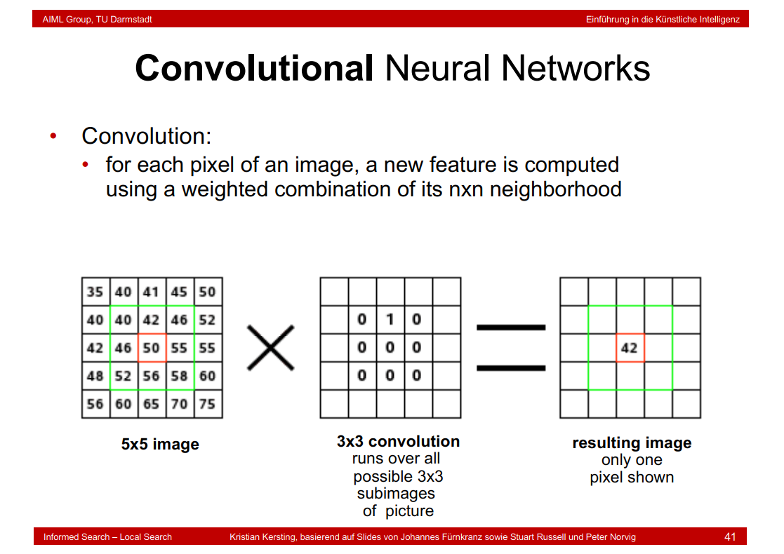
7.29 Convolutional Neural Networks
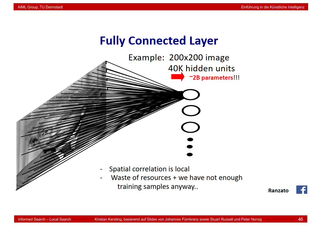
7.30 Fully Connected Layer
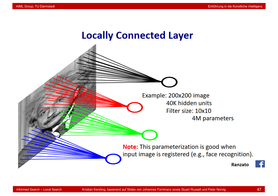
7.31 Locally Connected Layer
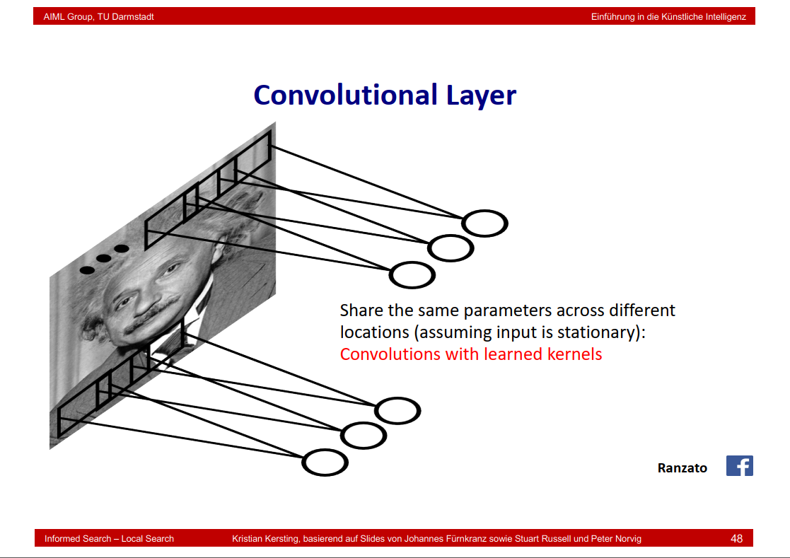
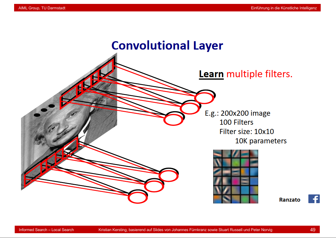
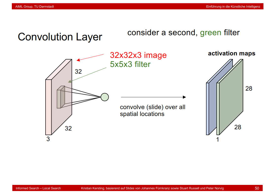
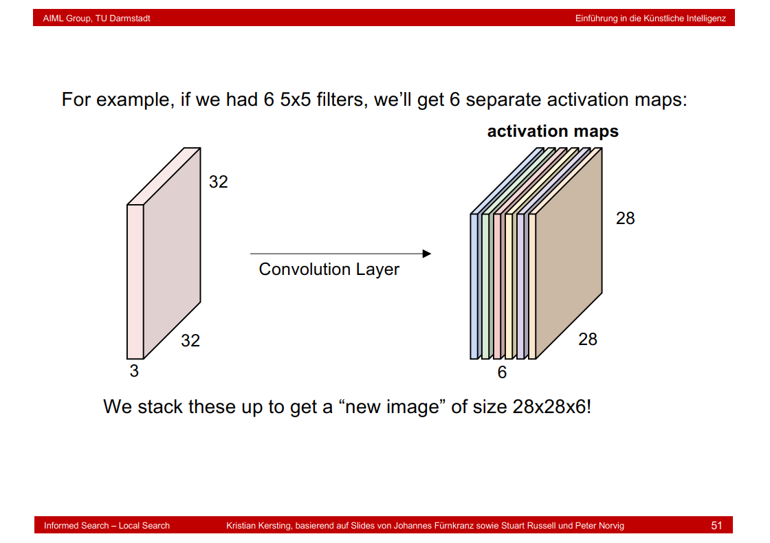
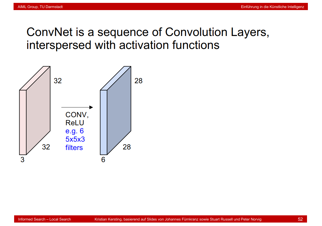
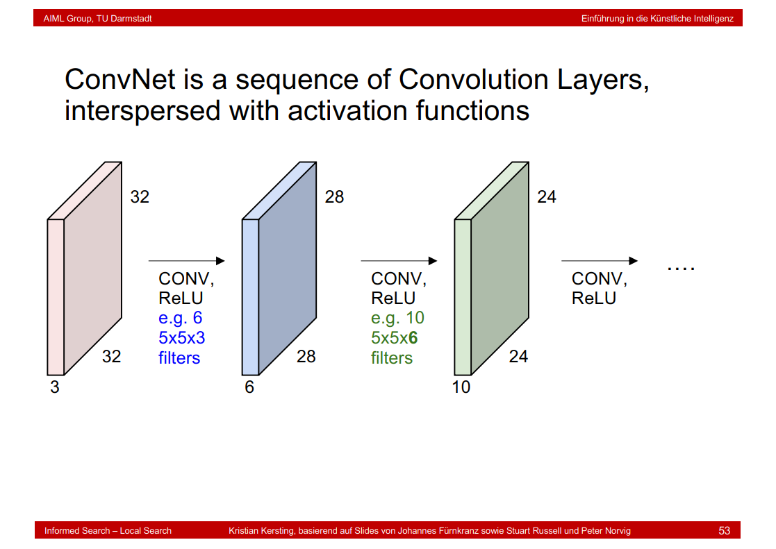
7.32 Convolutional Layer
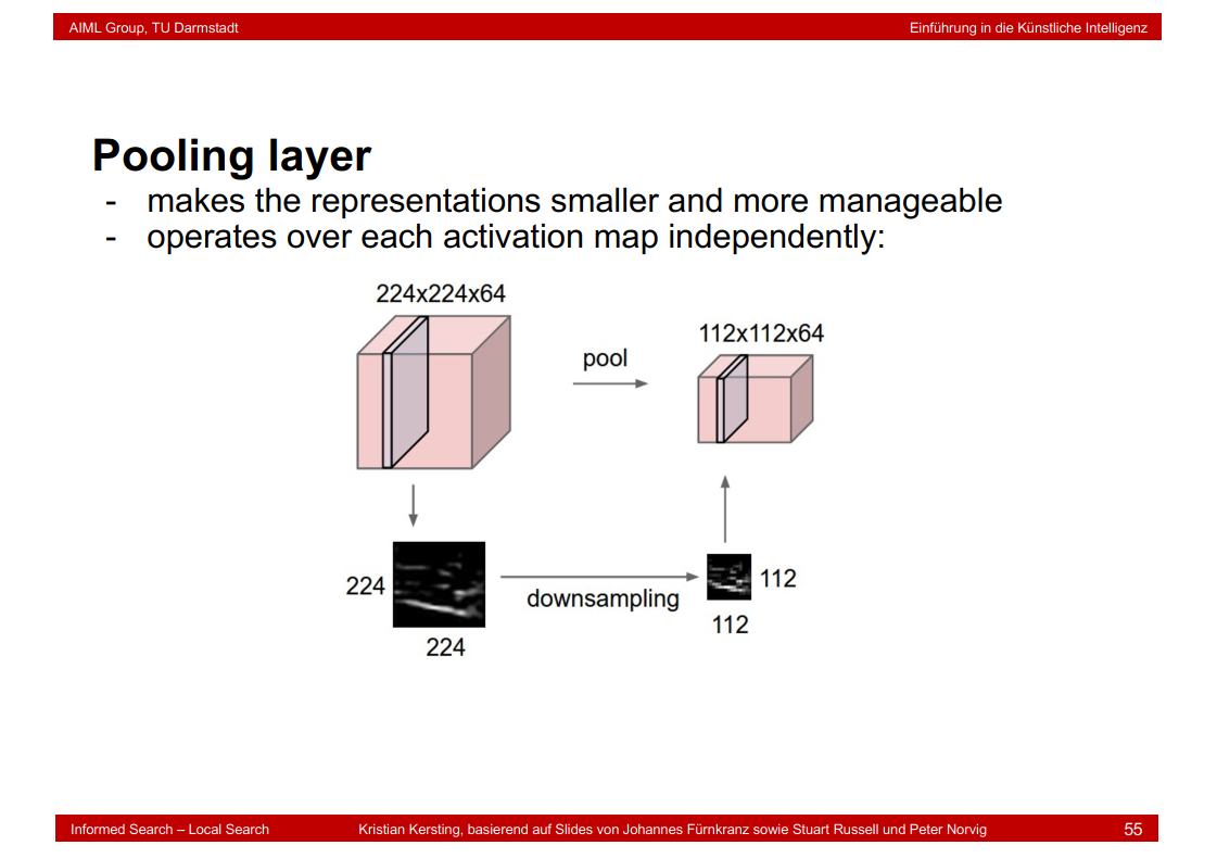
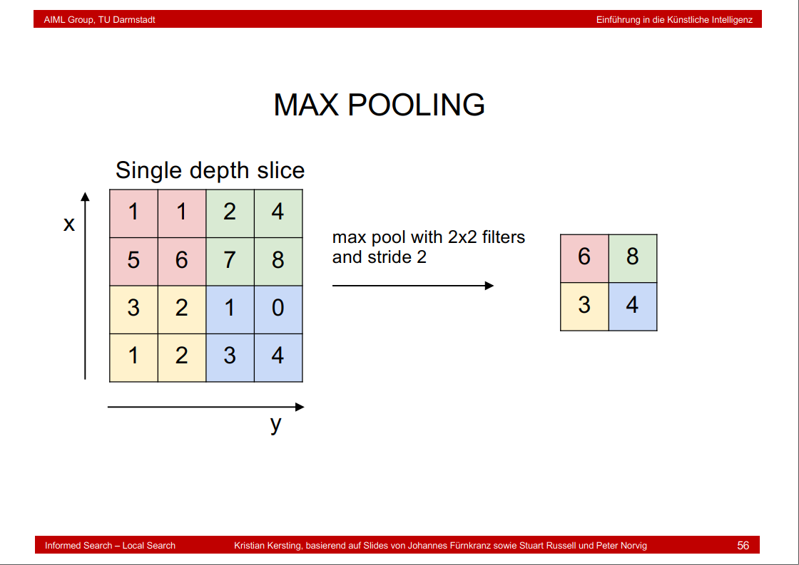
7.33 Pooling layer
7.34 There are many more architectures

8. Adversarial Search and Reinforcement Learning
8.1 Games vs. search problems

8.2 Game tree (2-player, deterministic, turns)
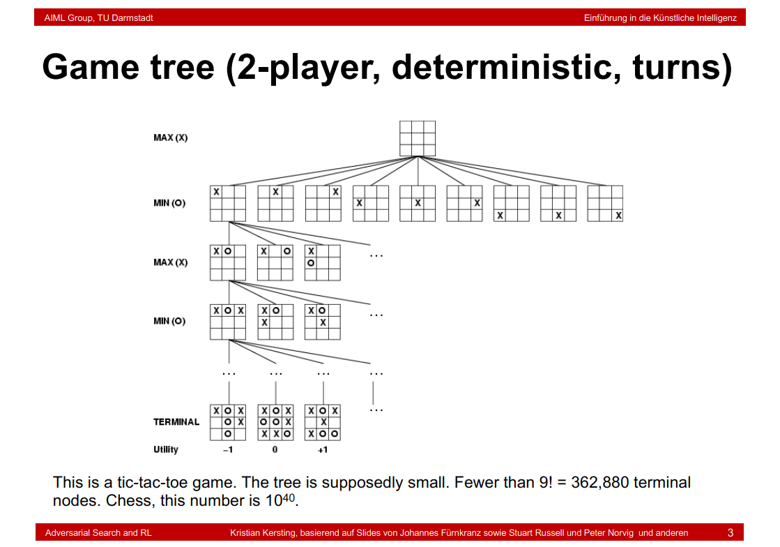
MIN(O)表示O的最小损失,MAX(X)表示X的最大获益,Terminal表示最终结果
补充:
Minimax算法又名极小化极大算法,是一种找出失败的最大可能性中的最小值的算法。Minimax算法常用于棋类等由两方较量的游戏和程序,这类程序由两个游戏者轮流,每次执行一个步骤。我们众所周知的五子棋、象棋等都属于这类程序,所以说Minimax算法是基于搜索的博弈算法的基础。该算法是一种零总和算法,即一方要在可选的选项中选择将其优势最大化的选择,而另一方则选择令对手优势最小化的方法。
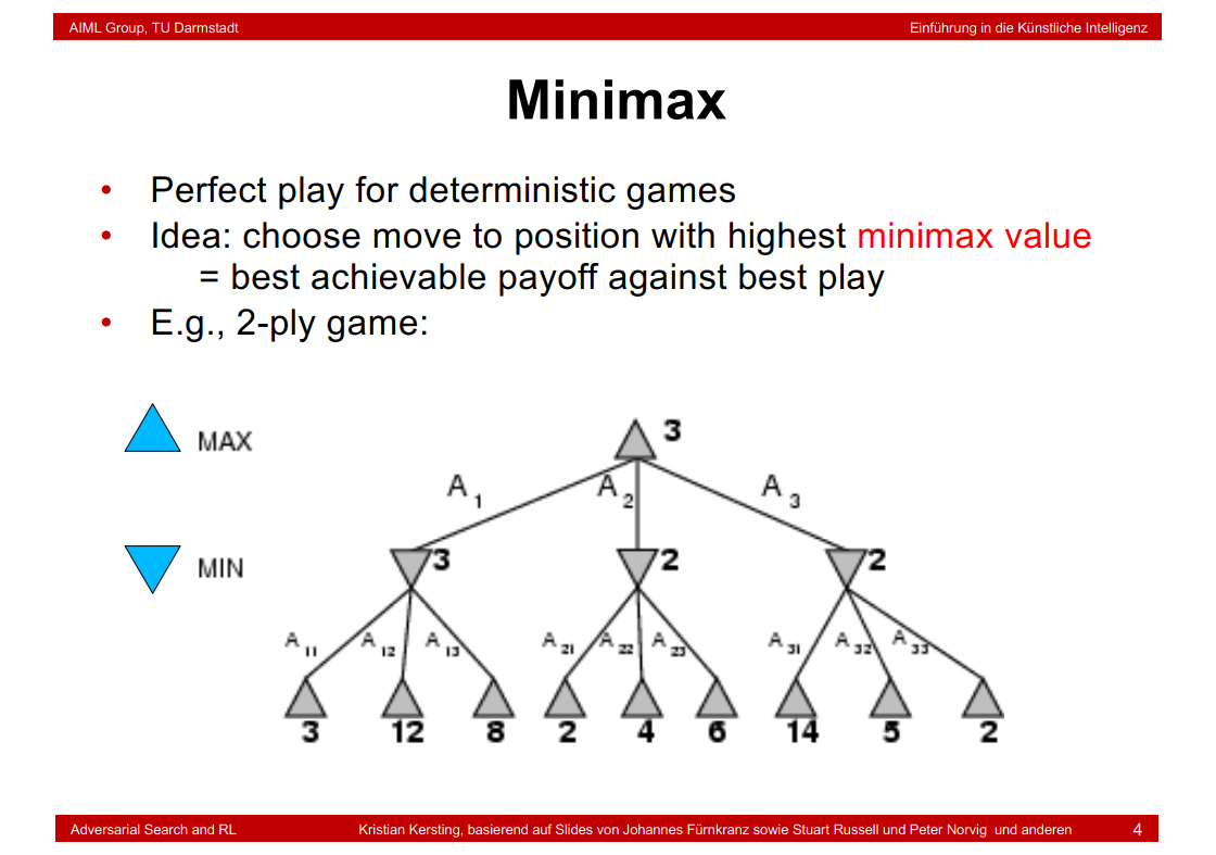
8.3 Minimax
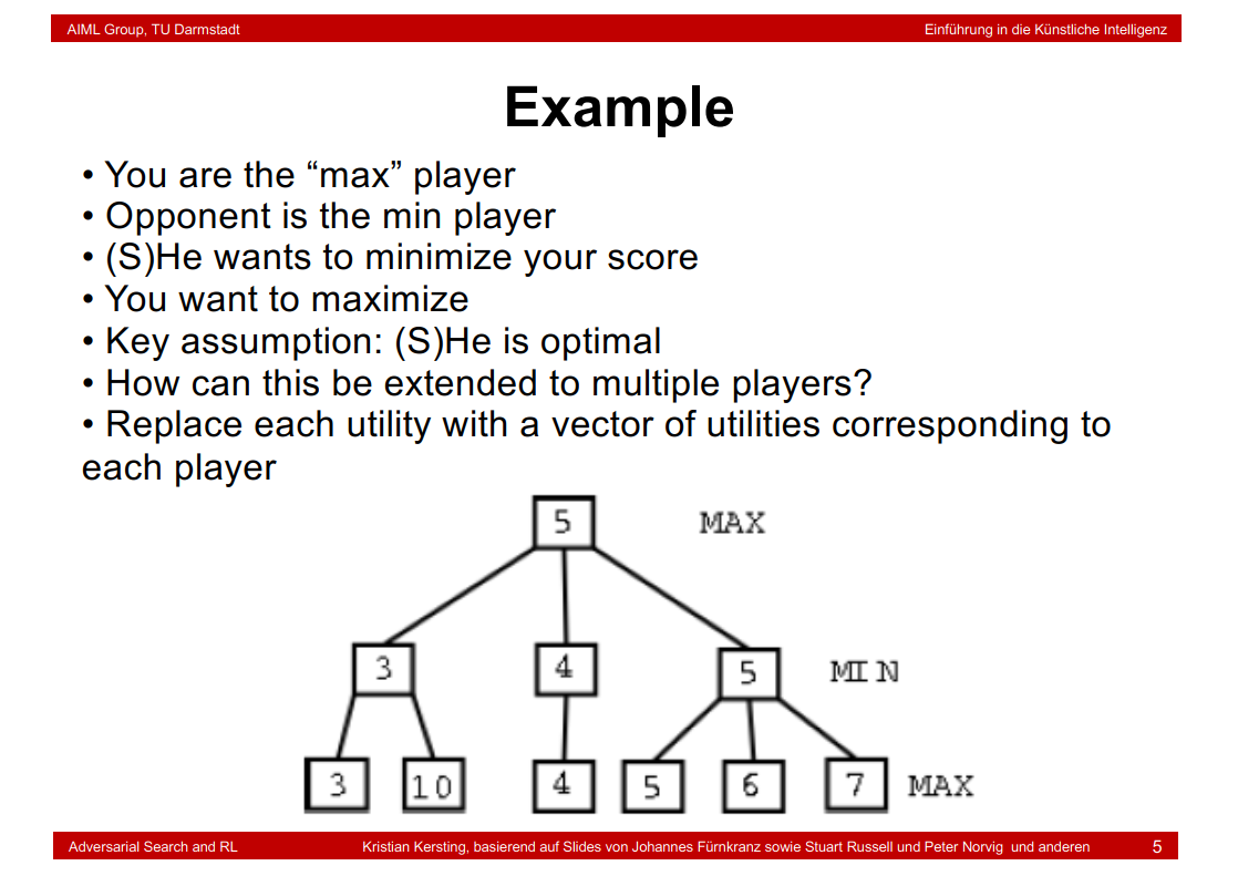
8.4 Example
补充:

minimax = 3
8.5 Properties of minimax
8.6 α-β pruning example
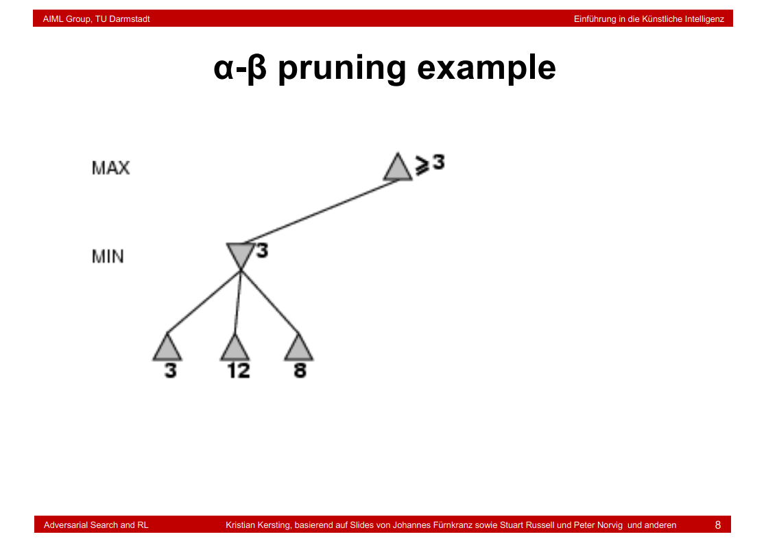
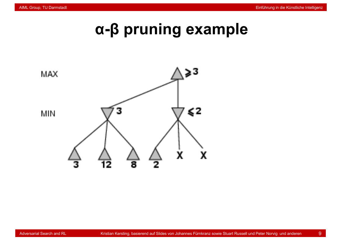
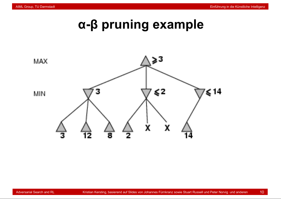
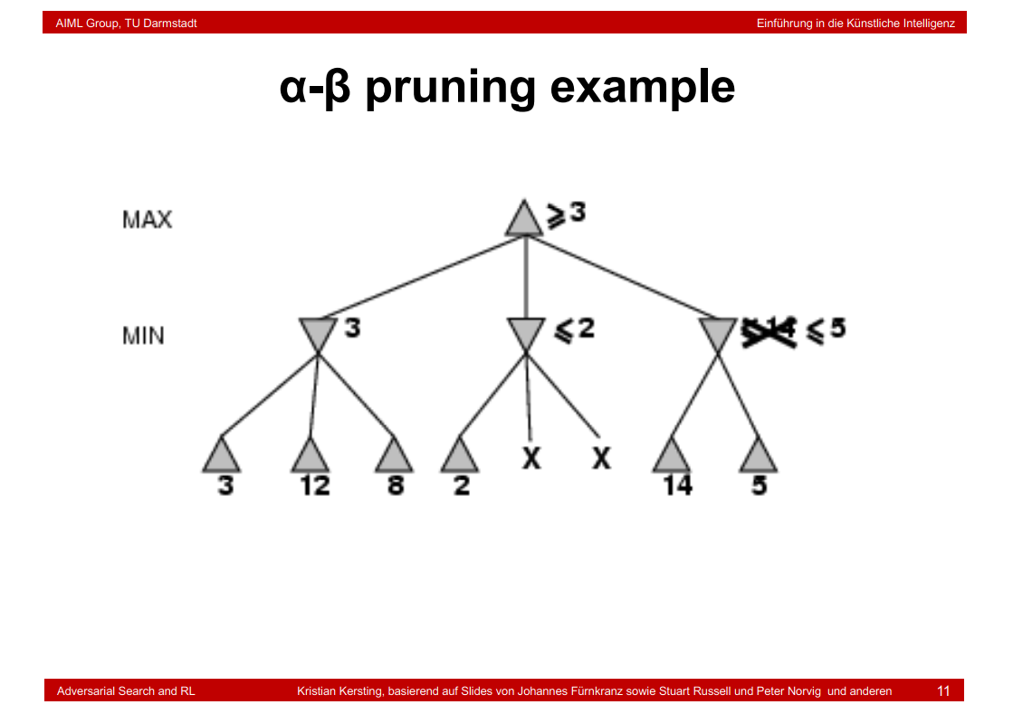
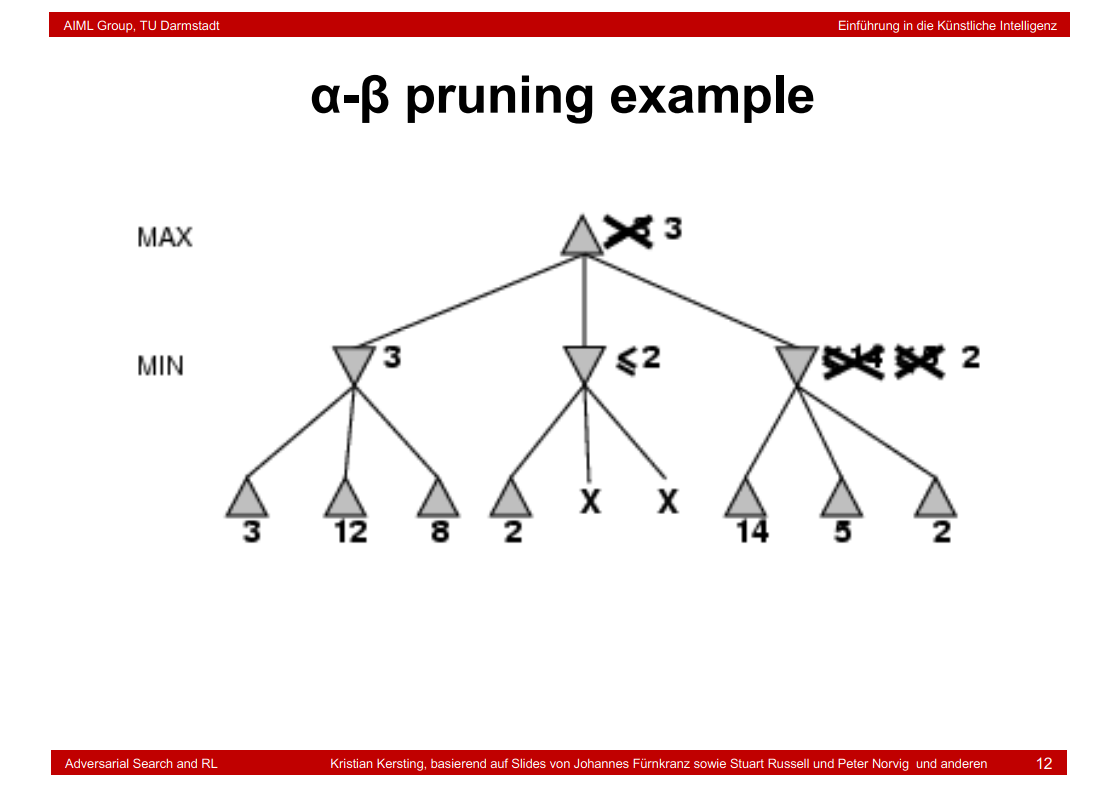
按步骤来的实例讲解:https://www.bilibili.com/video/BV1Bf4y11758
8.7 Why is it called α-β?

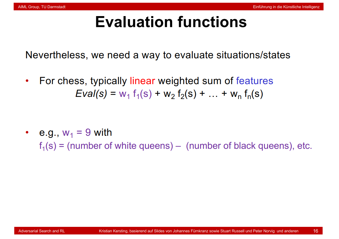
8.8 Evaluation functions
8.9 Reinforcement Learning
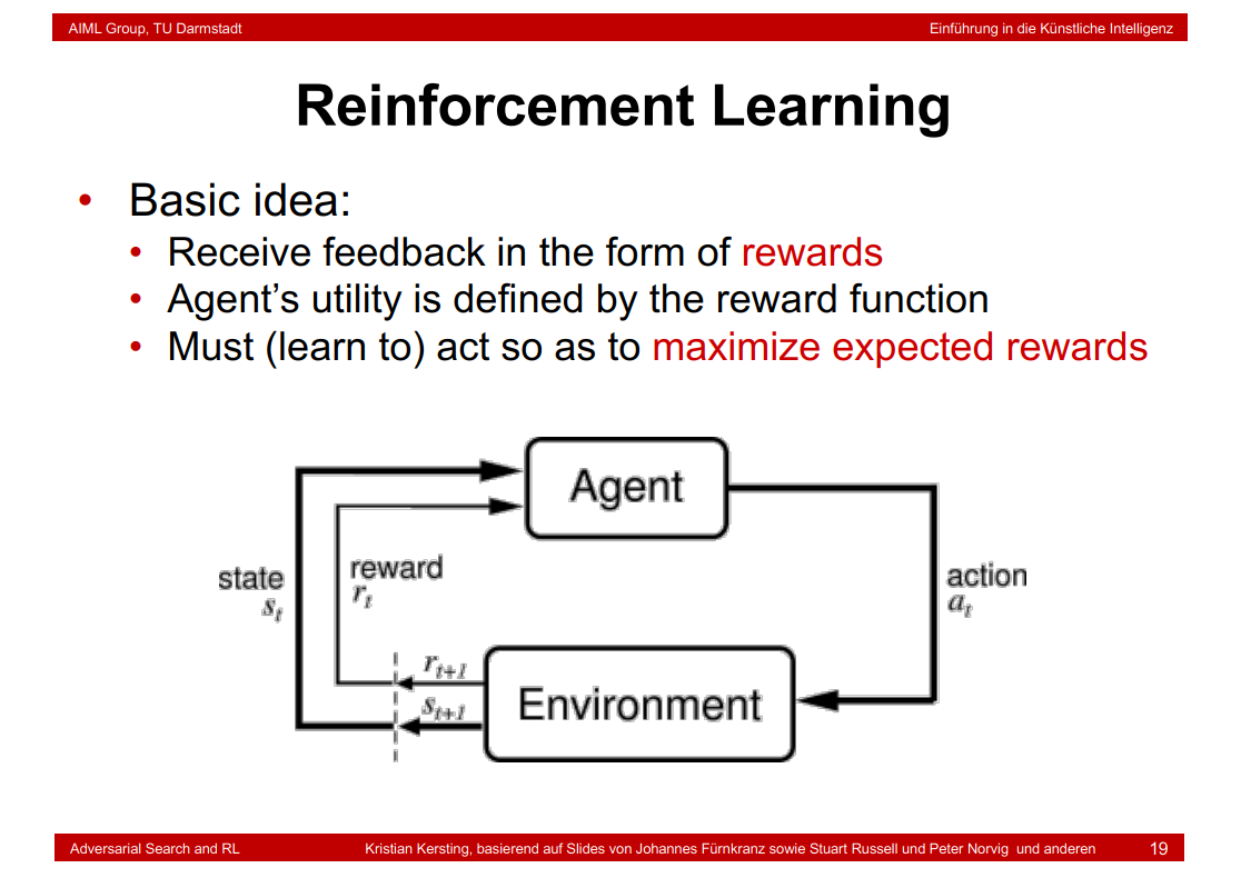
8.10 Reinforcement Learning (RL)

8.11 Credit Assignment Problem

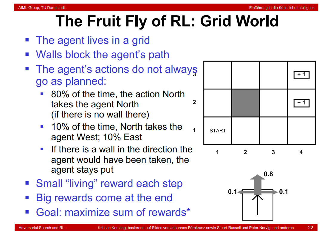
8.12 The Fruit Fly of RL: Grid World
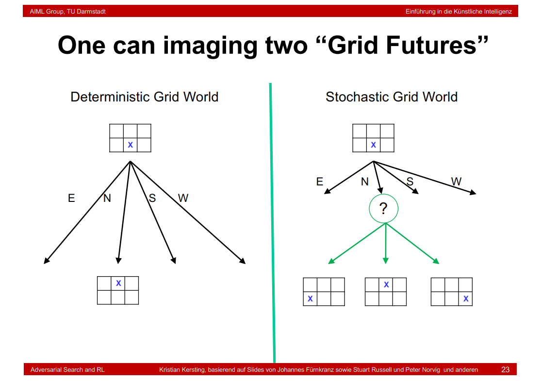
8.13 One can imagine two “Grid Futures”
8.14 Now, what are Markov Decision Processes (MDP)?
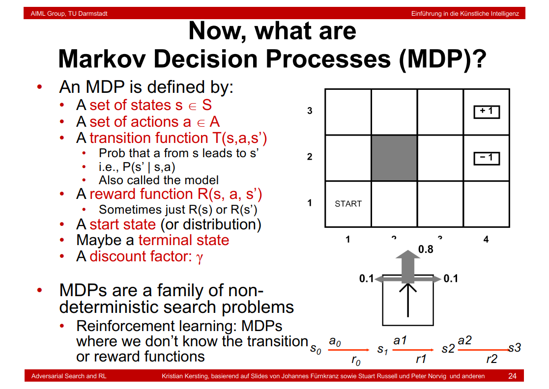
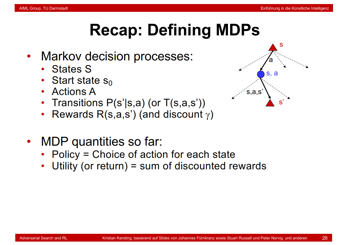
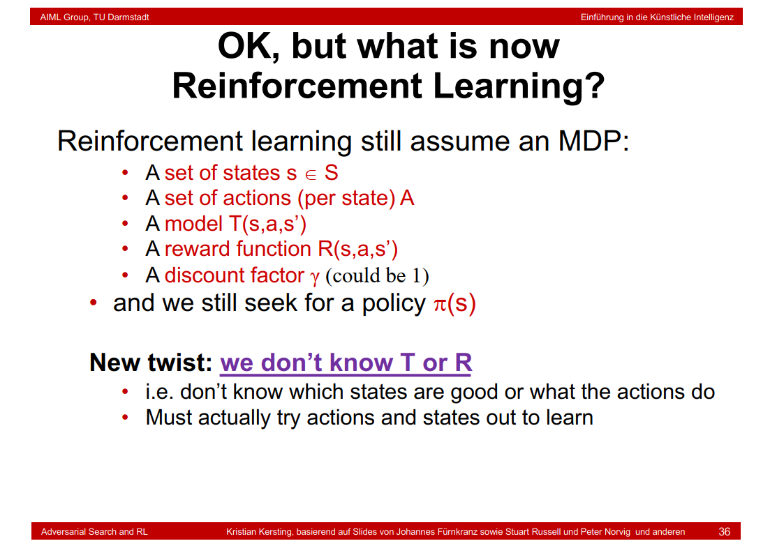
要说强化学习,就必须说说马尔科夫决策过程 (Markov Decision Processes, MDP)。马尔可夫决策过程是基于马尔可夫过程理论的随机动态系统的决策过程,其分五个部分:
S 表示状态集 (States);
A 表示动作集 (Actions);
P(s' | s, a) or T(s, a, s') 表示状态 s 下采取动作 a 之后转移到 s' 状态的概率;
R(s, a) 表示状态 s 下采取动作 a 获得的奖励;
γ 是衰减因子,在0-1之间。
链接:https://www.jianshu.com/p/20a16735f0bc
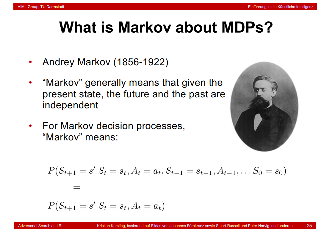
8.15 What is Markov about MDPs?
8.16 What does it mean to solve MDPs?

在强化学习当中,我们通过优化期望回报函数来优化动作策略,从而使得机器人习得最优策略到达目的地。正式的,我们定义π为状态集合映射到动作集合A的策略,即S -> A。也就是在某个状态s中,我们通过最优策略π选择最好的动作a(即a = π(s)),获得更好的回报。
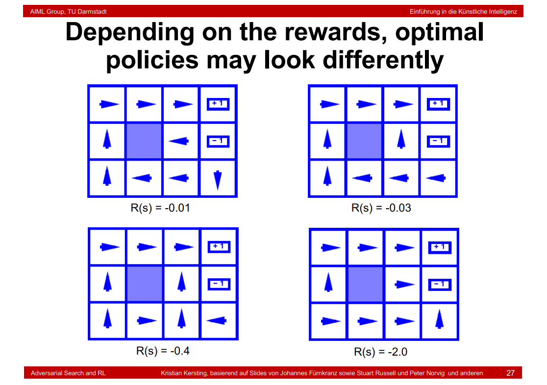
R(s, a, s') = -0.03表示惩罚,是自定义的值
8.17 Depending on the rewards, optimal policies may look differently
8.18 Recap: Defining MDPs
8.19 Intuition of Action Selection
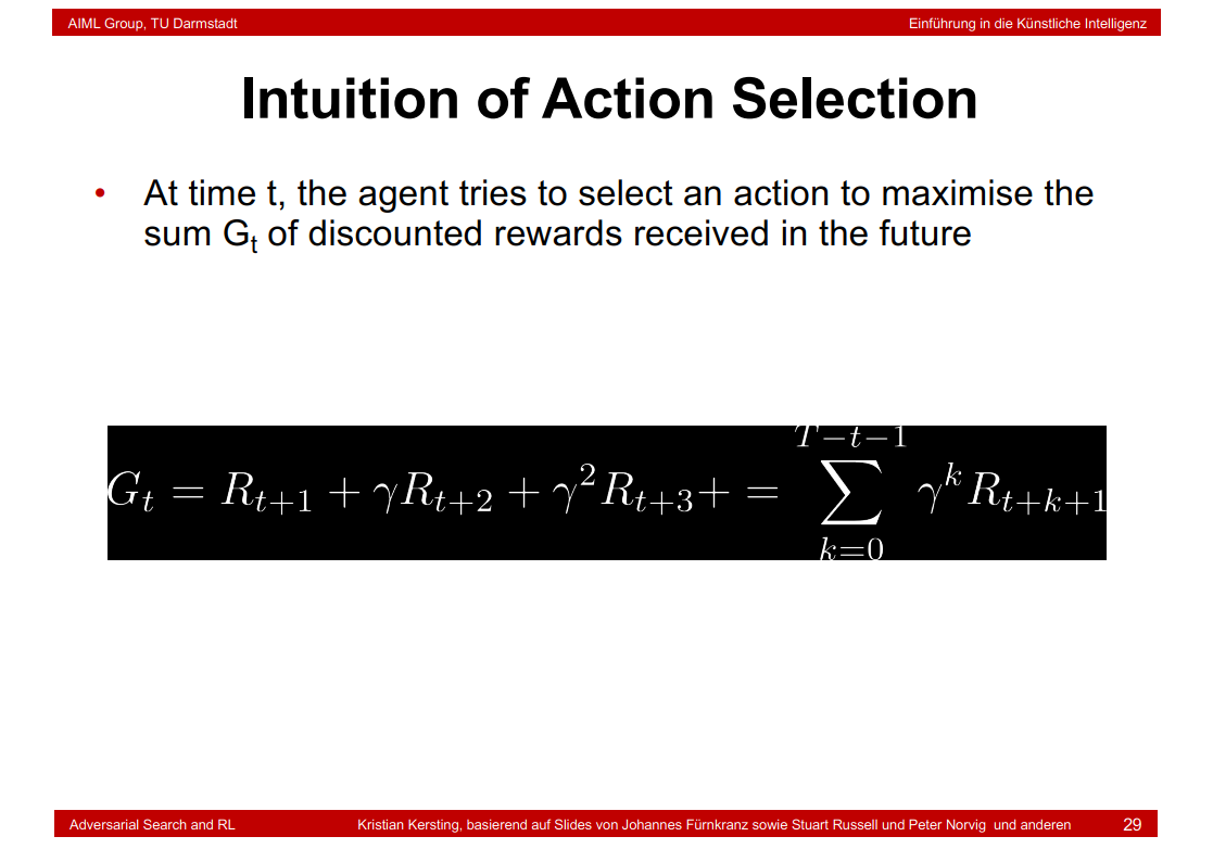
这里的γ是衰退因子,其目的是让机器人尽快获得高的回报,尽量晚的或者高的惩罚。γ越小越要求机器人快速得到回报。
8.20 Why Discounted Rewards

8.21 Optimal Utilities
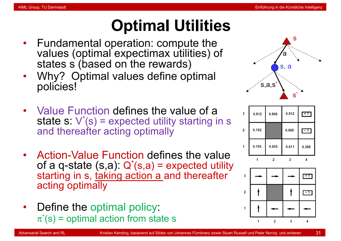
Q(1,3) = 0.8×0.66+0.1×0.388+0.1×0.655 = 0.6323
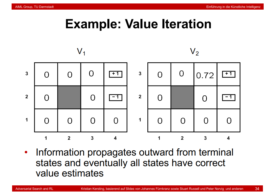
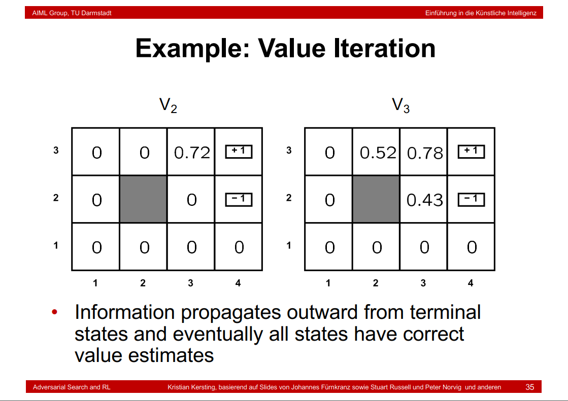
第一个表+1和-1表示reward的值,灰色表示该区域不可以行走。
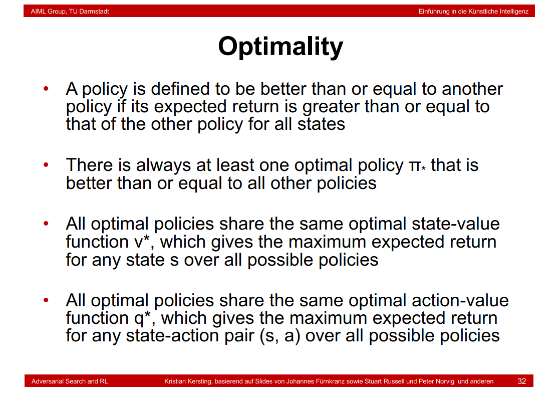
8.22 Optimality
8.23 How can we compute, eg, the value function? Value Iteration

8.24 Example: Value Iteration
8.25 OK, but what is now Reinforcement Learning?
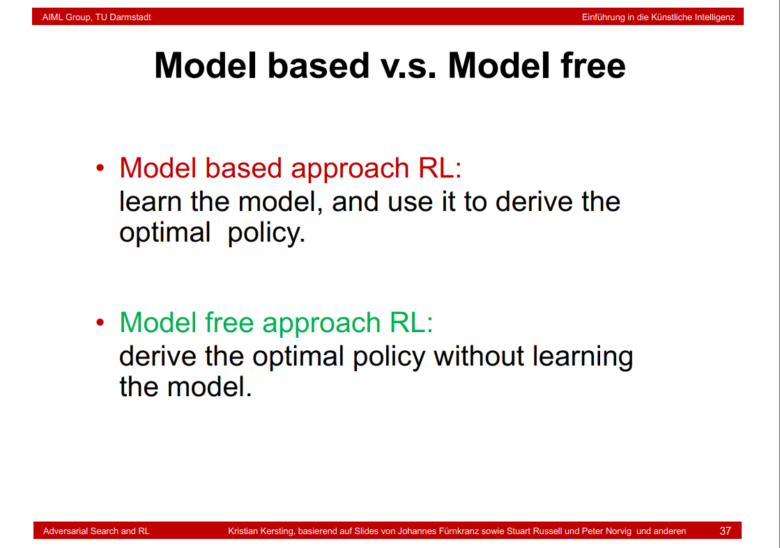
8.26 Model based v.s. Model free
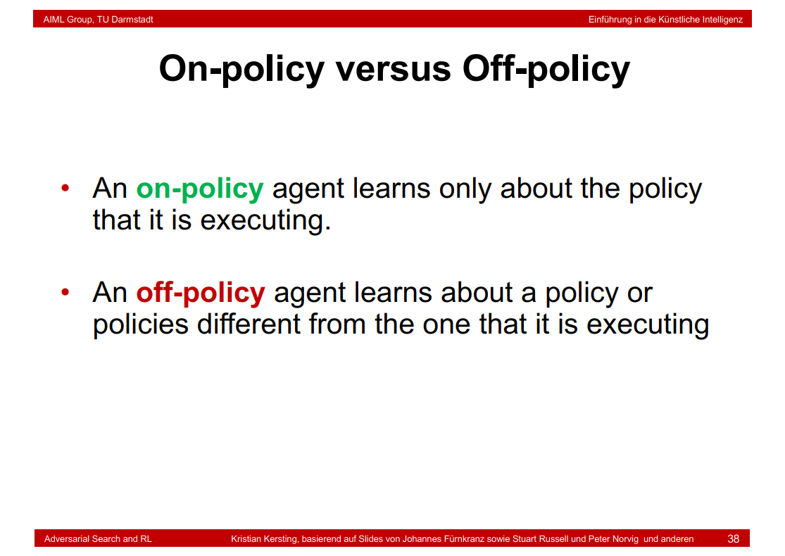
8.27 On-policy versus Off-policy
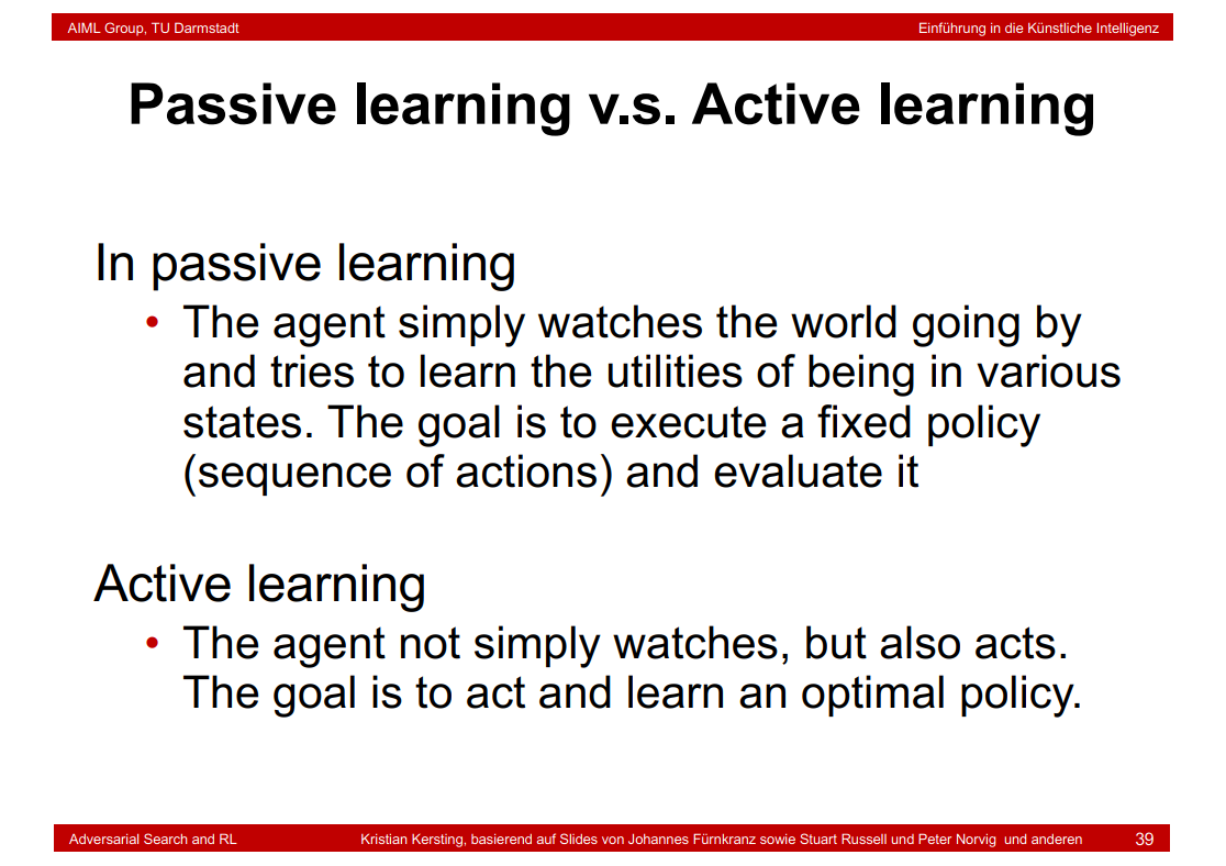
8.28 Passive learning v.s. Active learning
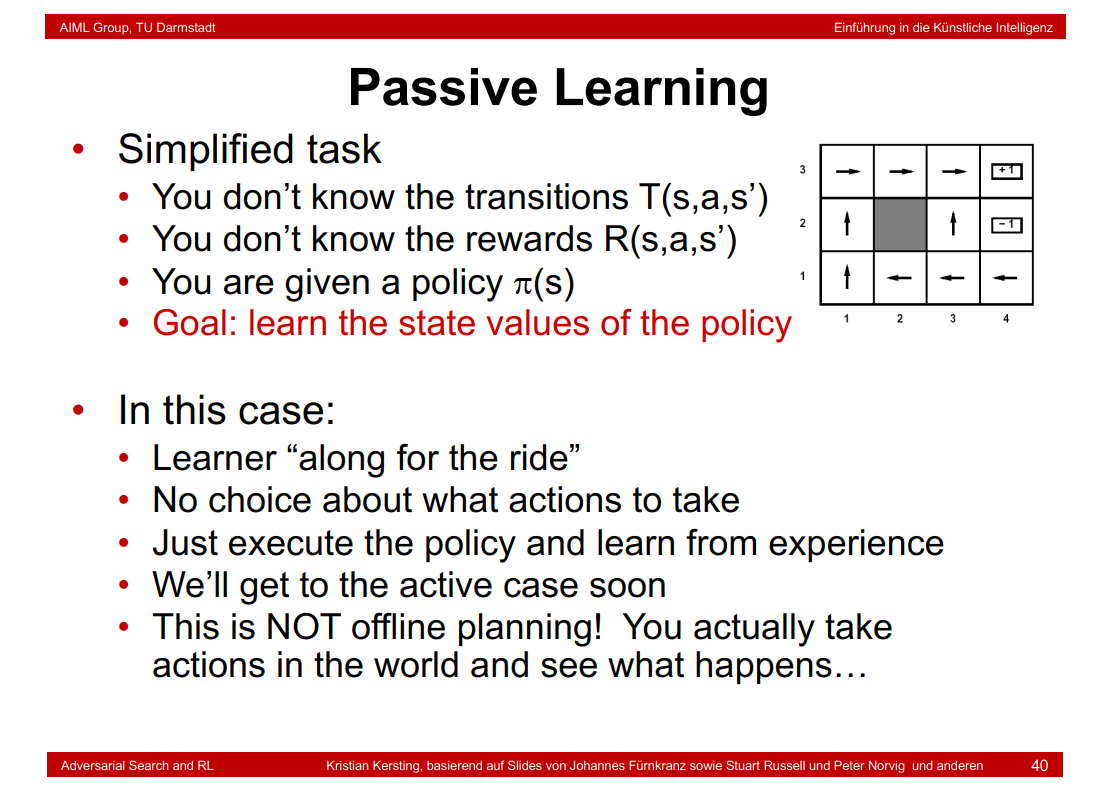
8.29 Passive Learning
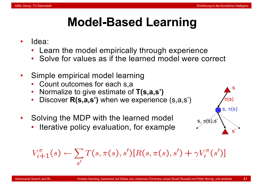
8.30 Model-Based Learning
8.31 Sample-Based Policy Evaluation?

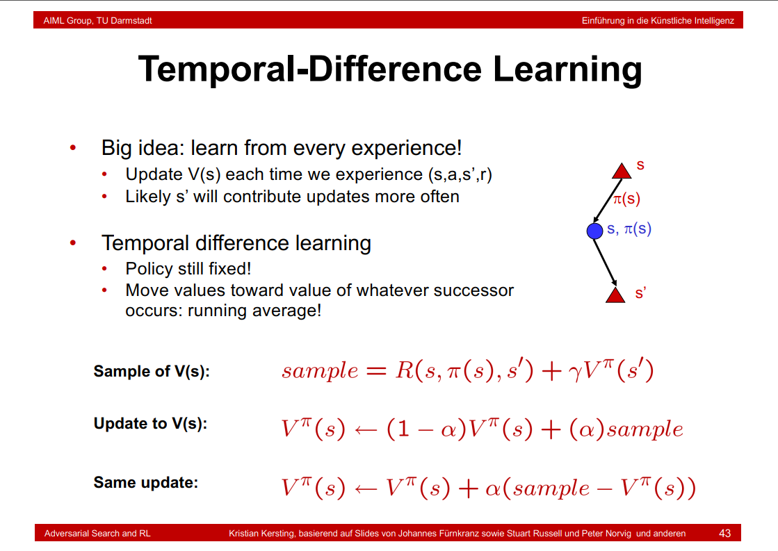
8.32 Temporal-Difference Learning
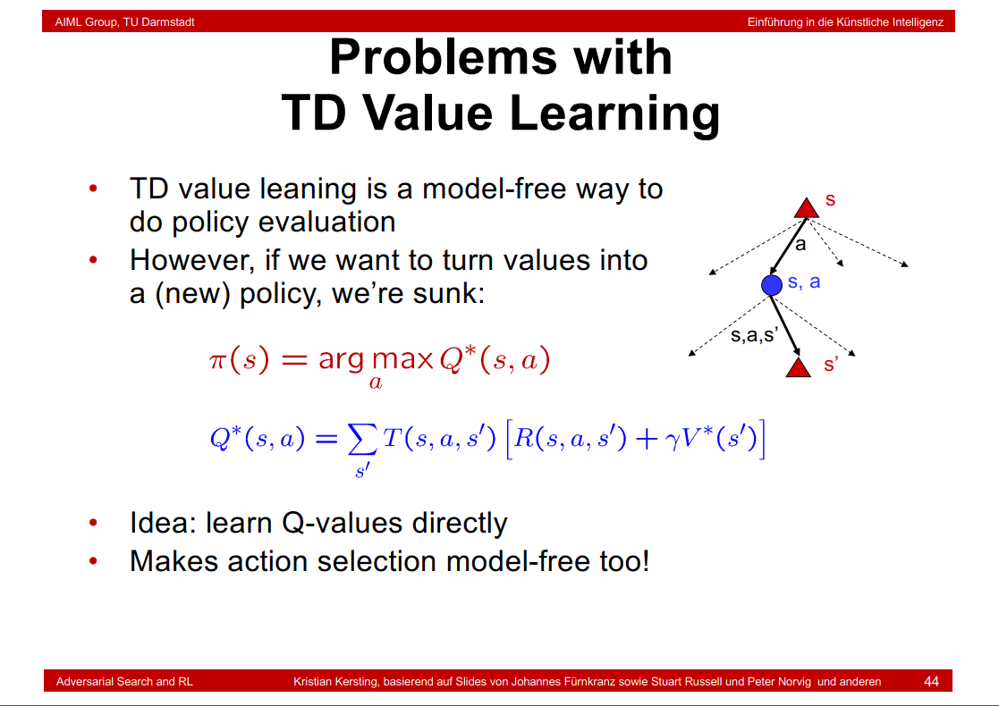
8.33 Problems with TD Value Learning
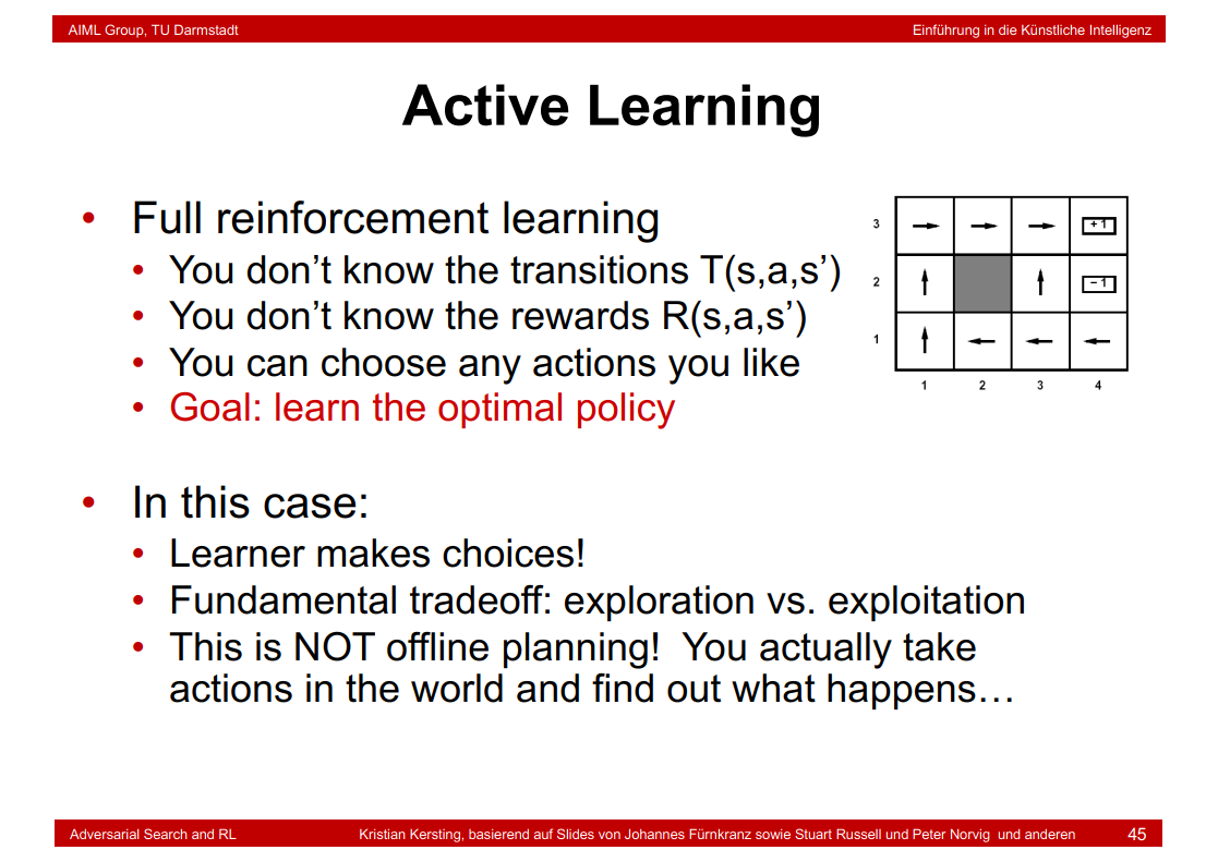
8.34 Active Learning
8.35 Q-Learning

其中α为学习速率(learning rate),γ为折扣因子(discount factor)。根据公式可以看出,学习速率α越大,保留之前训练的效果就越少。折扣因子γ越大,maxQ(s',a')所起到的作用就越大。maxQ(s',a')指的是记忆中的利益,
R是眼前的利益,即reward矩阵。
详细解释:https://blog.csdn.net/itplus/article/details/9361915
8.36 Q-Learning Properties
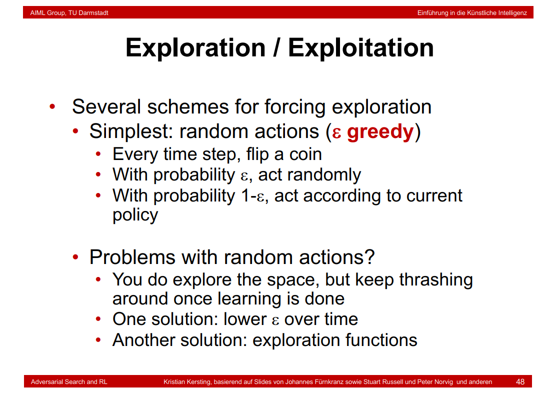
8.37 Exploration / Exploitation
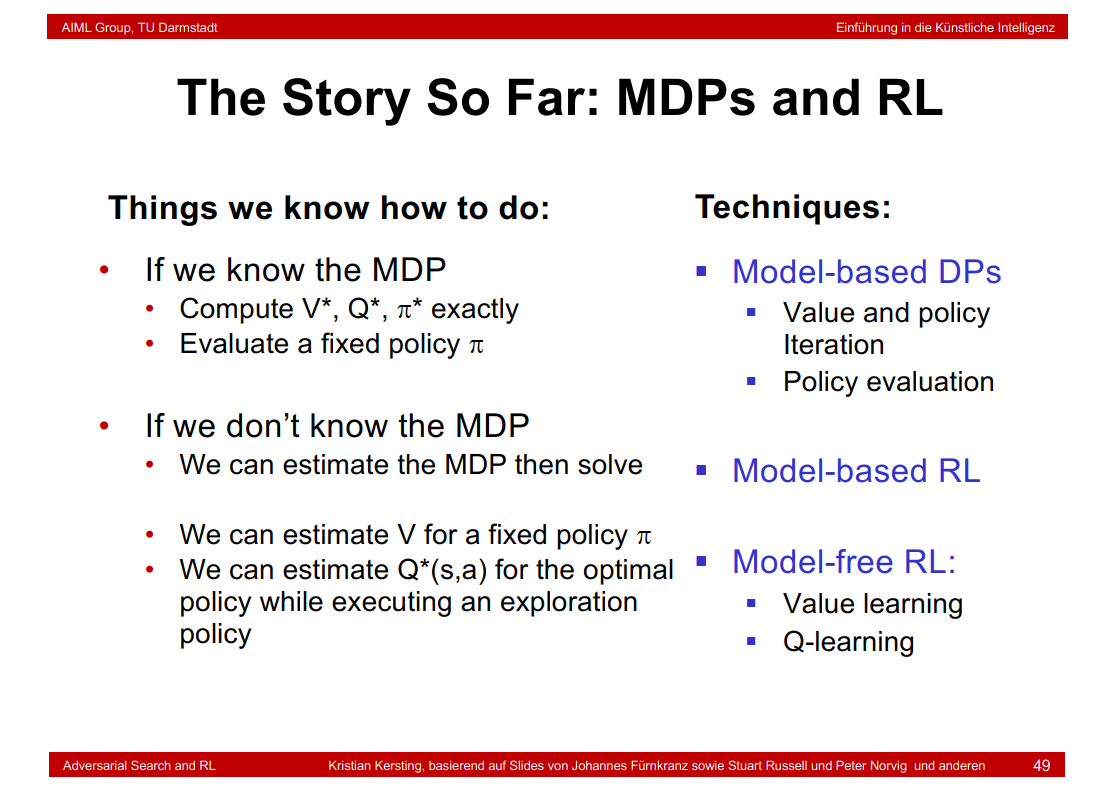
8.38 The Story So Far: MDPs and RL
8.39 Q-Learning in realistic domains
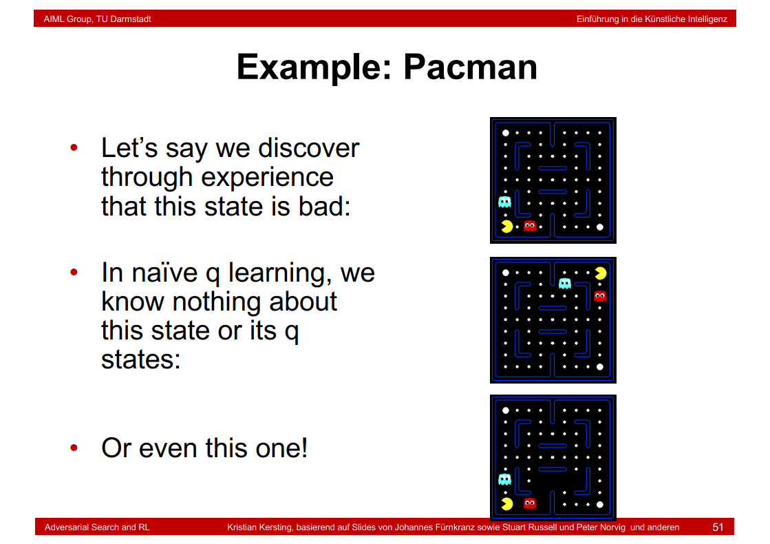
8.40 Example: Pacman
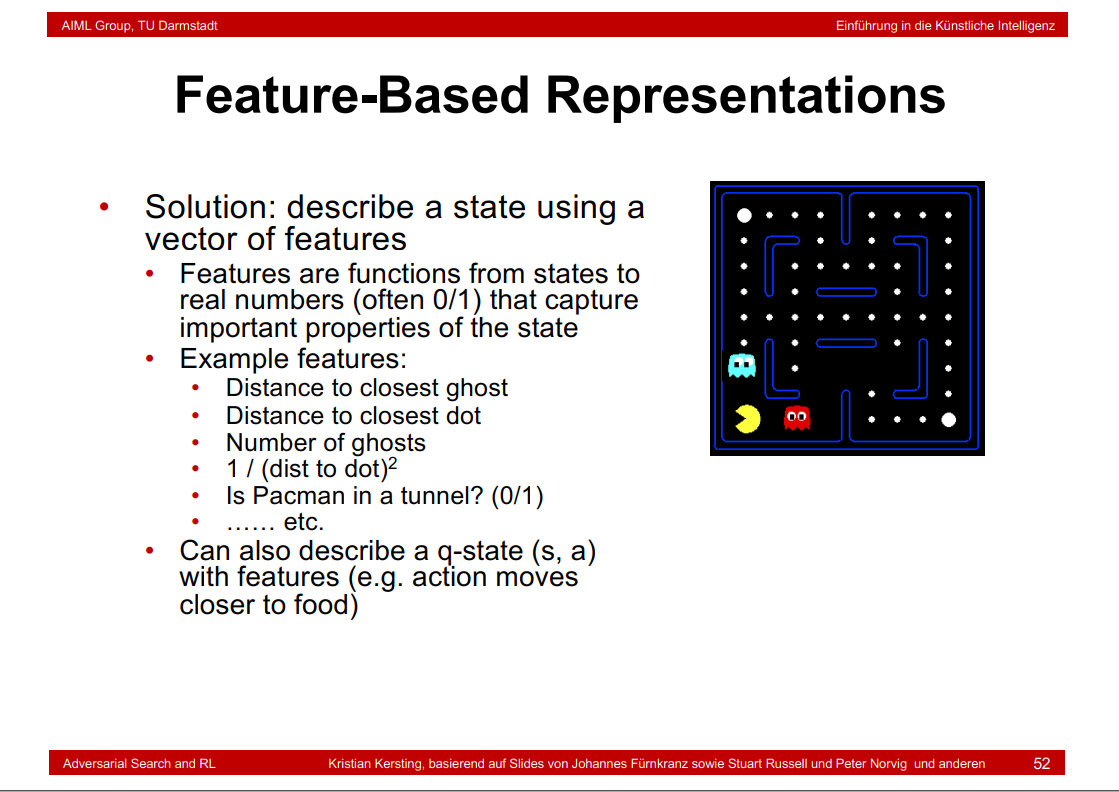
8.41 Feature-Based Representations
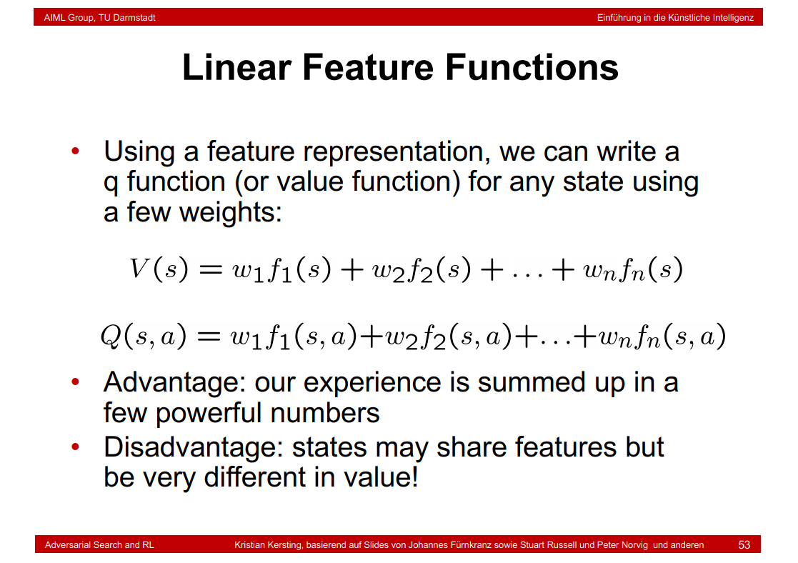
8.42 Linear Feature Functions
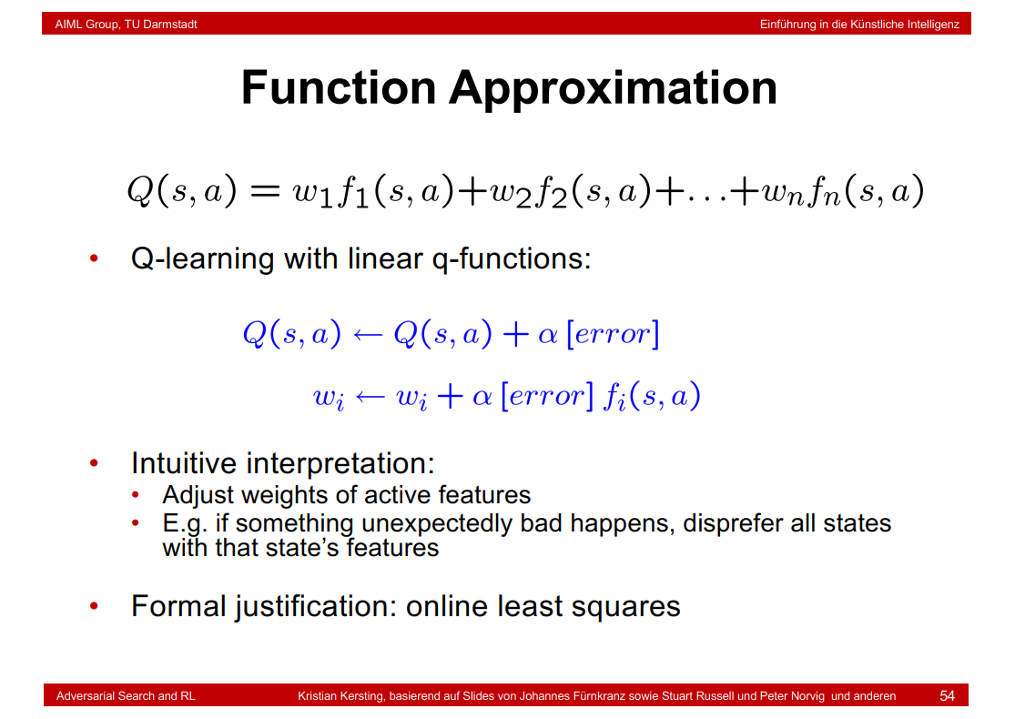
8.43 Function Approximation
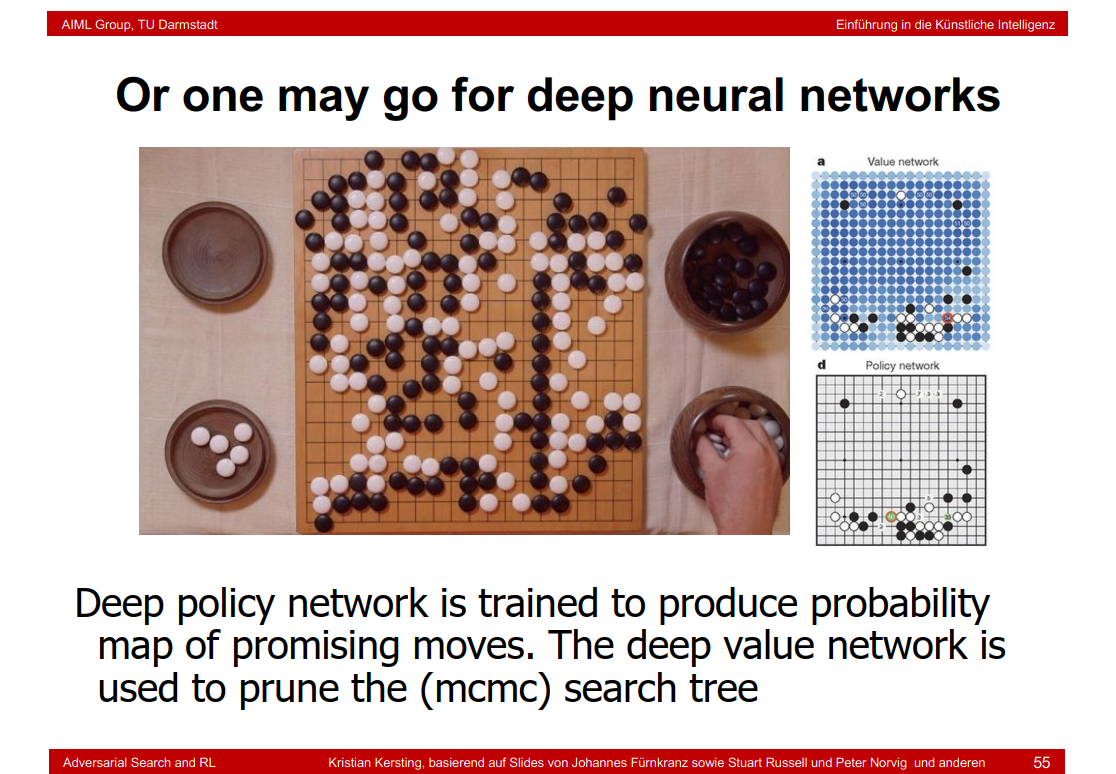
8.44 Or one may go for deep neural networks
8.45 Deep Q-Networks (DQN)
8.46 Policy Search

9. Uncertainty and Bayesian Networks
9.1 Uncertain Actions

9.2 Problems with Uncertainty
9.3 Probabilities
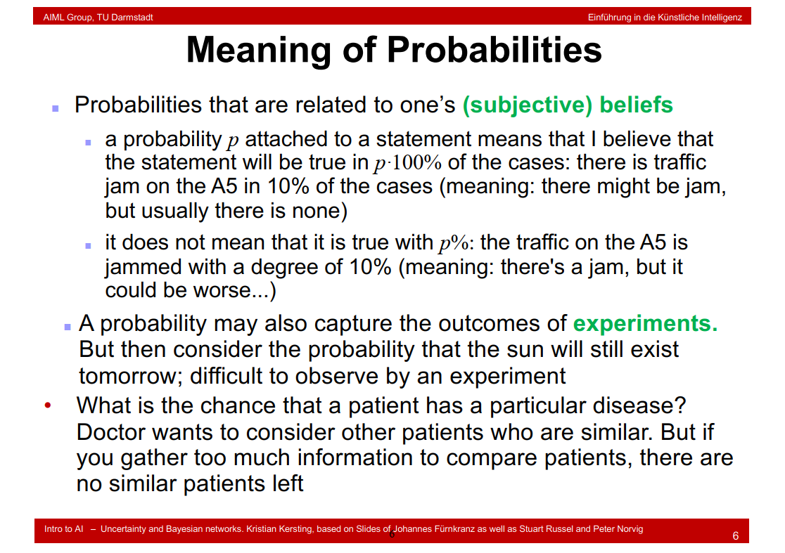
9.4 Meaning of Probabilities
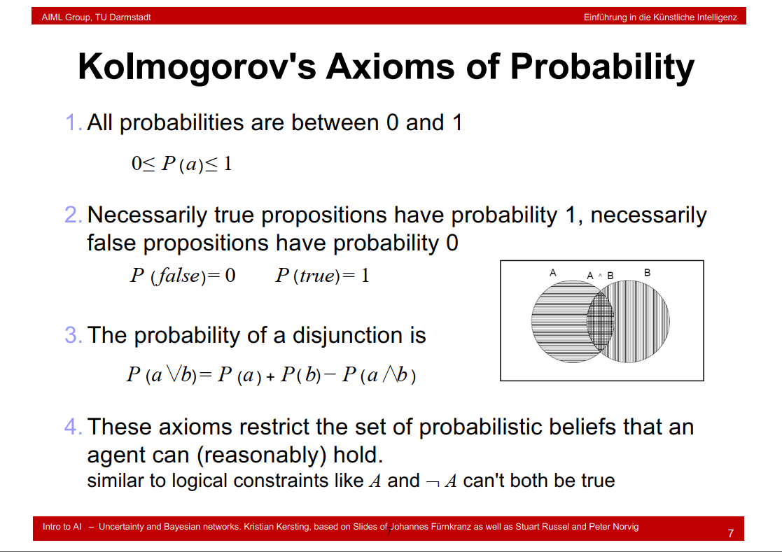
9.5 Kolmogorov's Axioms of Probability
9.6 Violation of Axioms of Probability
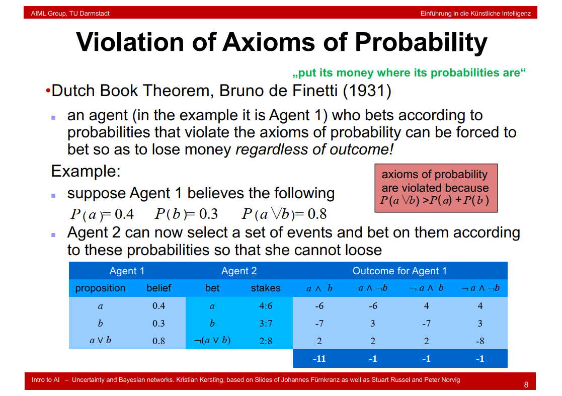
a∩b为什么是-6???
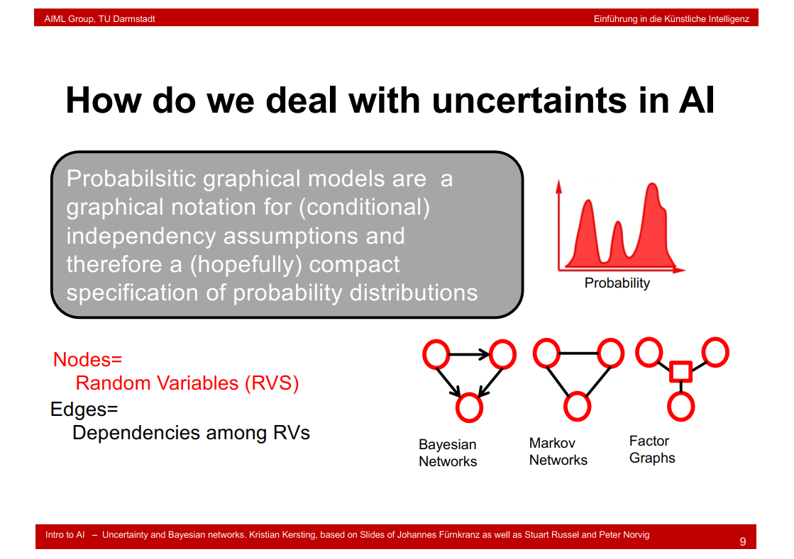
9.7 How do we deal with uncertaints in AI
9.8 Discrete Random Variables
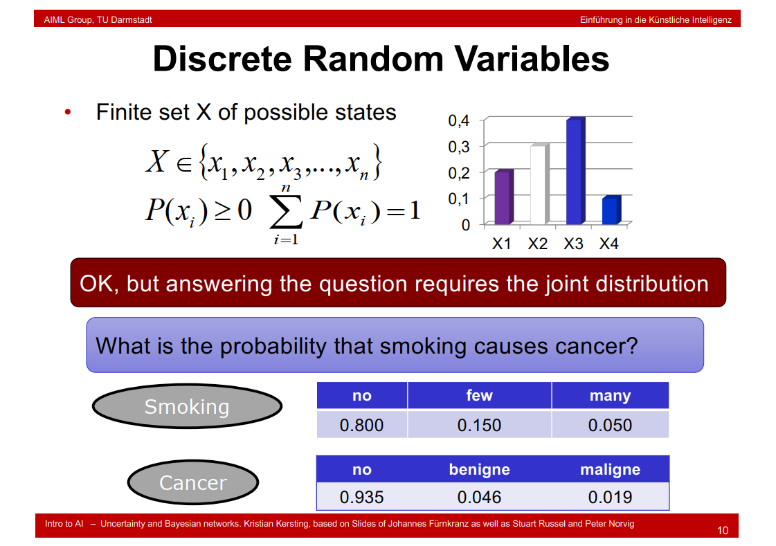
benign:良性; malign:恶性
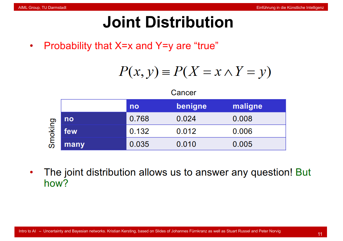
9.9 Joint Distribution
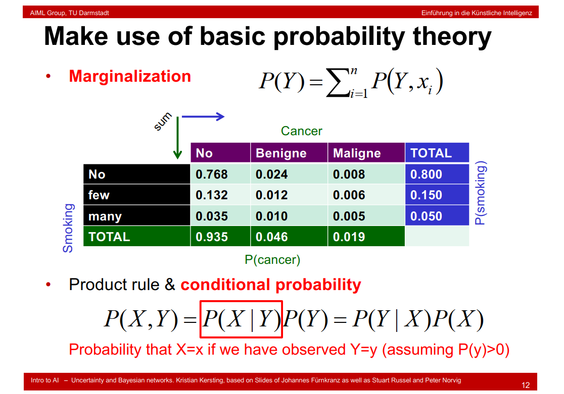
9.10 Make use of basic probability theory
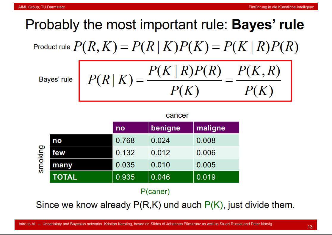
9.11 Probably the most important rule: Bayes’ rule
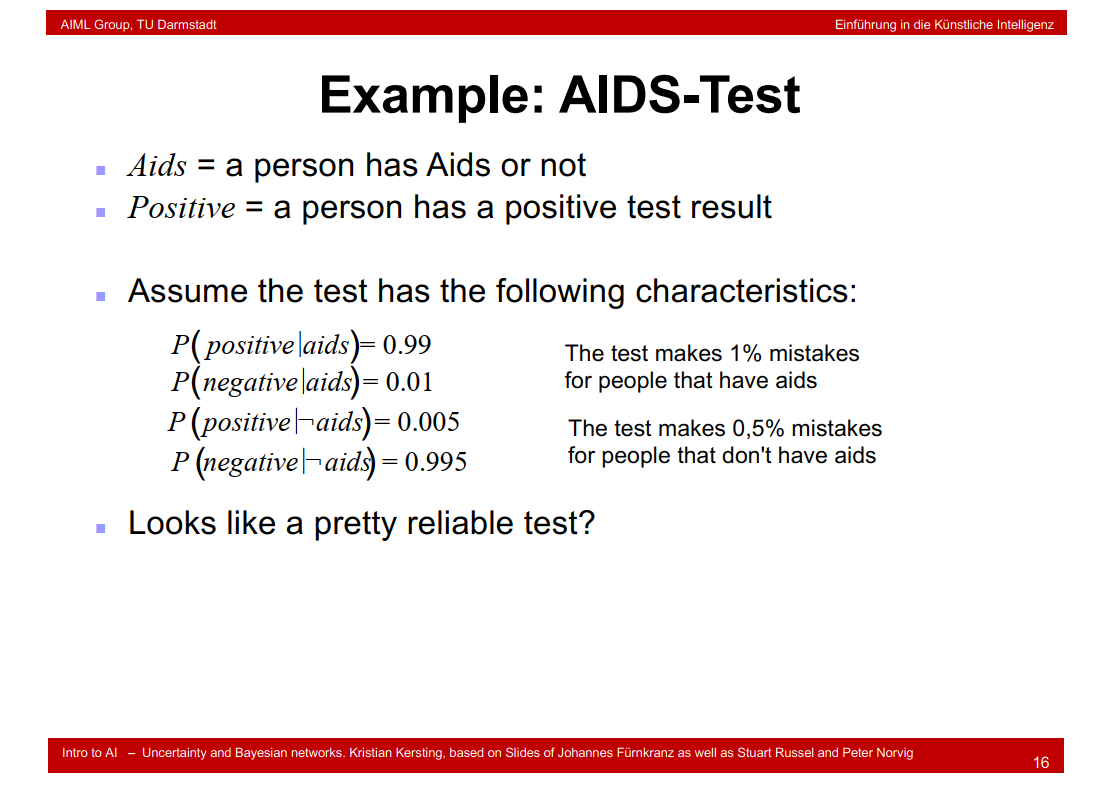
9.12 Example: AIDS-Test

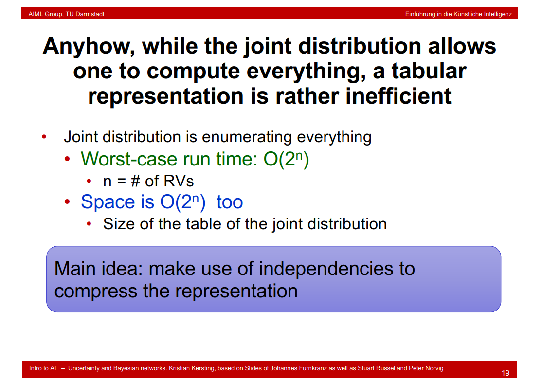
9.13 inefficient tabular representation
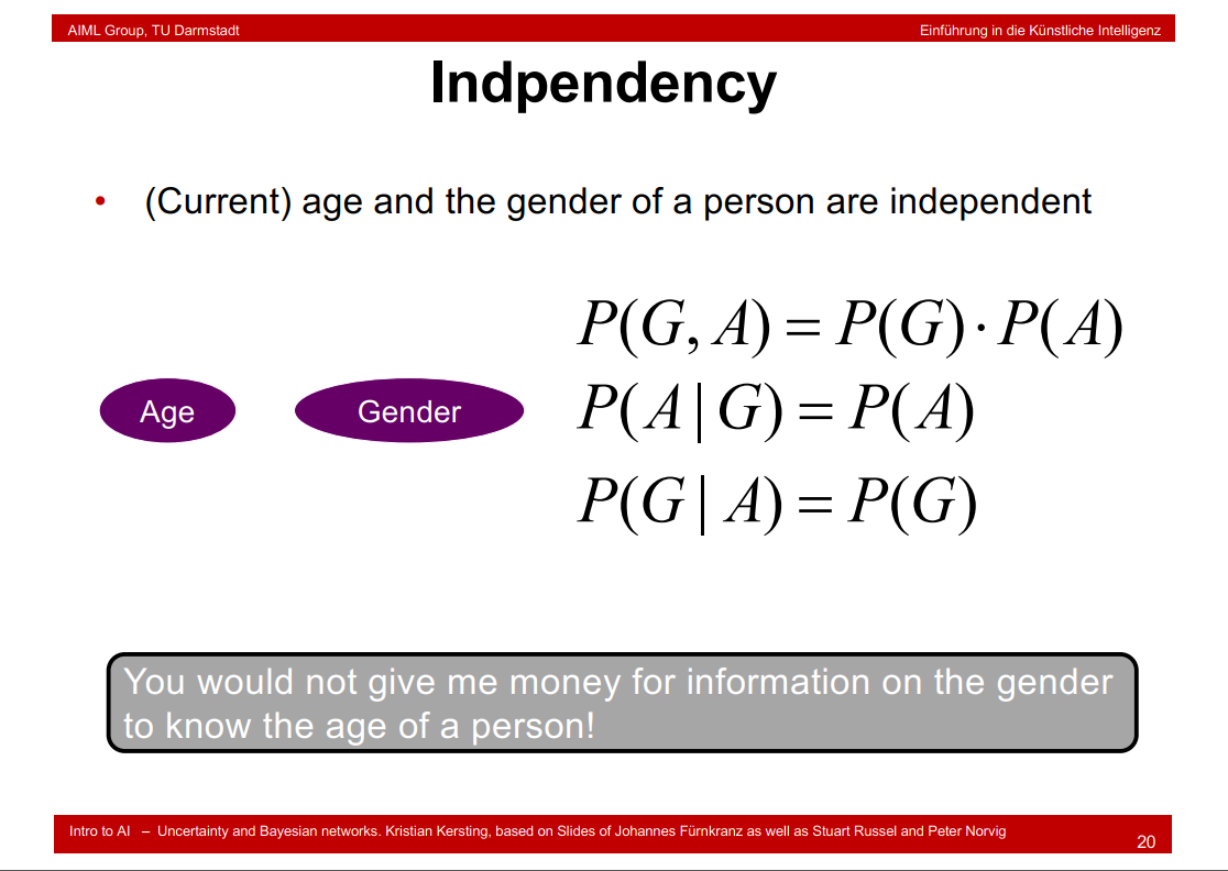
9.14 Indpendency
9.15 Conditional Independence

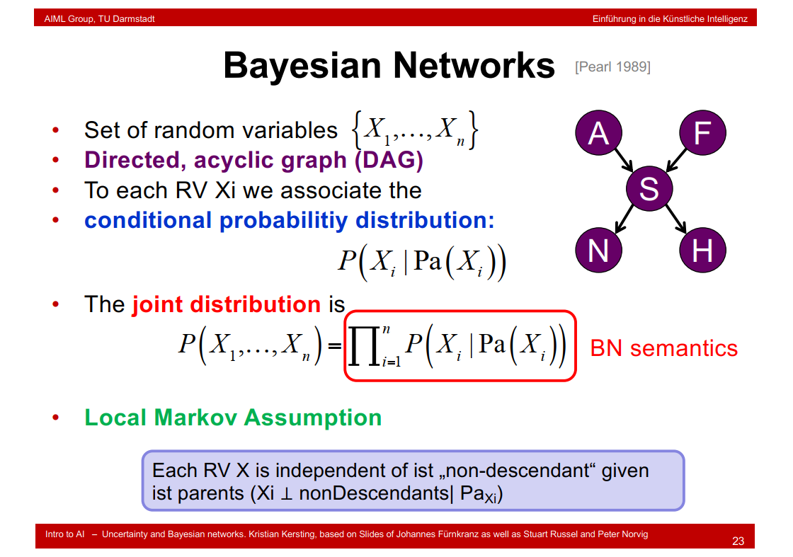
9.16 Bayesian Networks
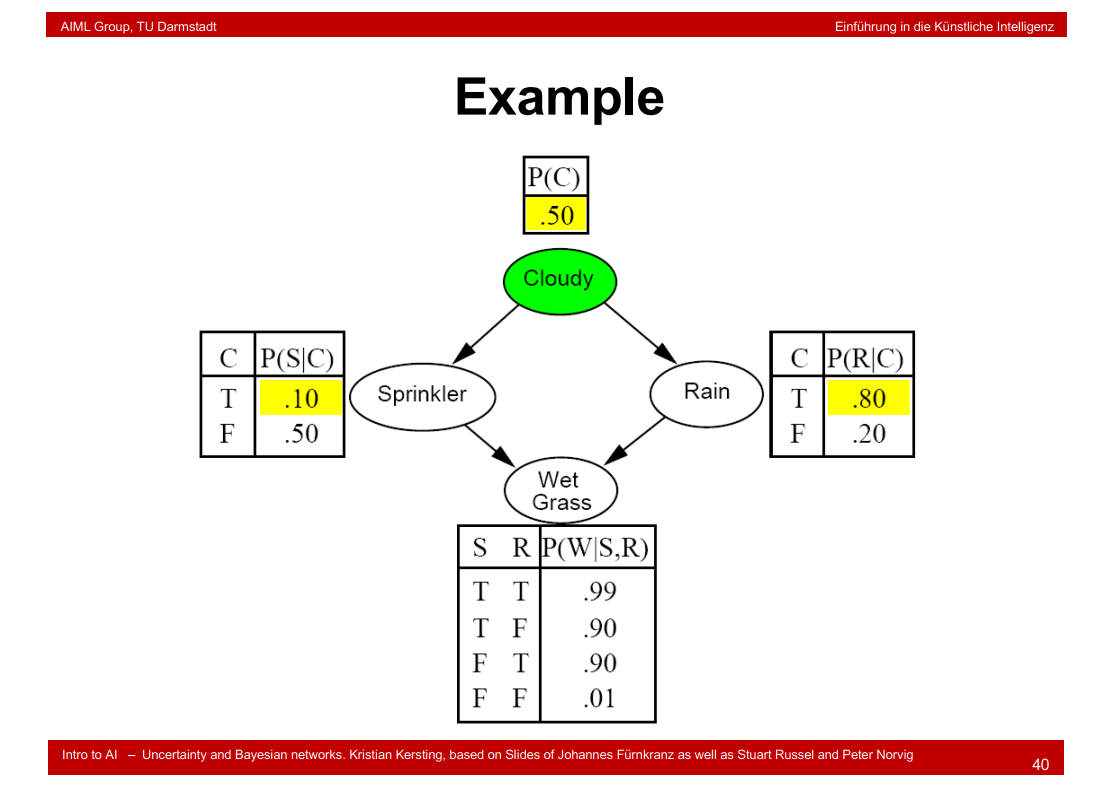
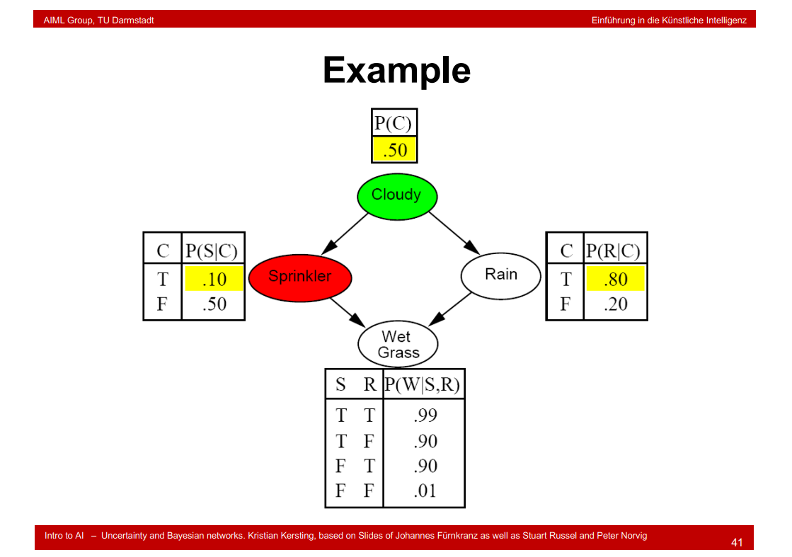
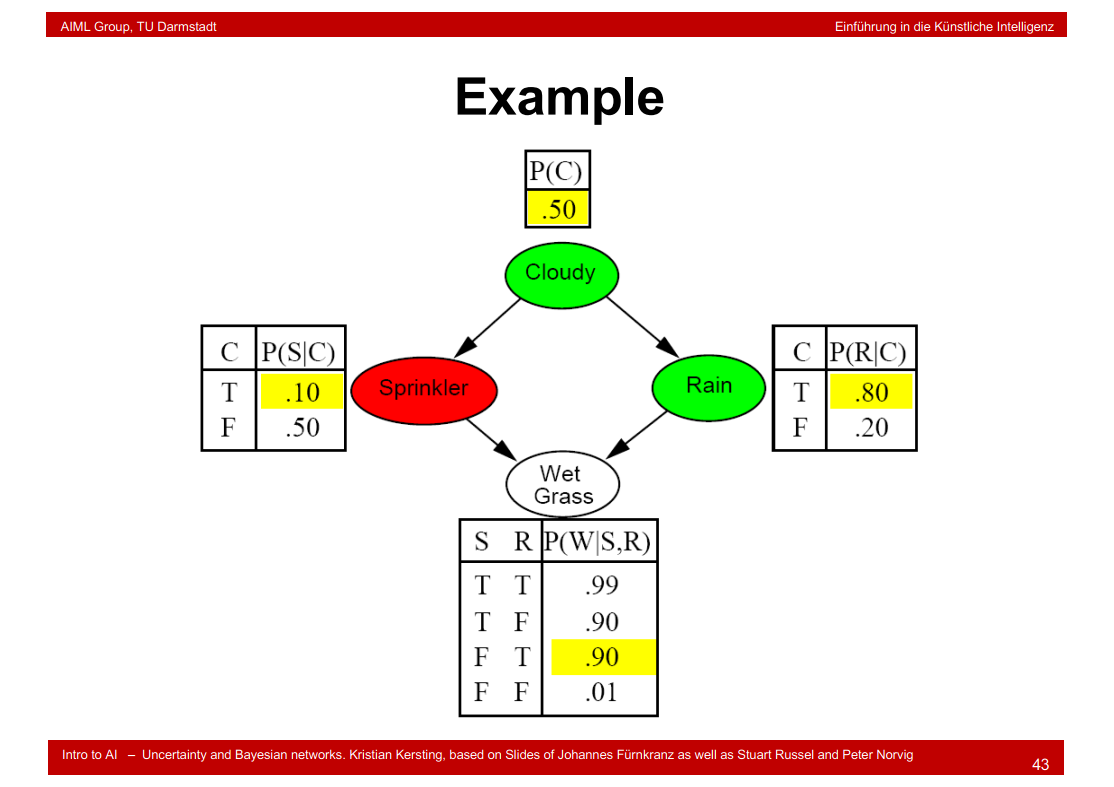
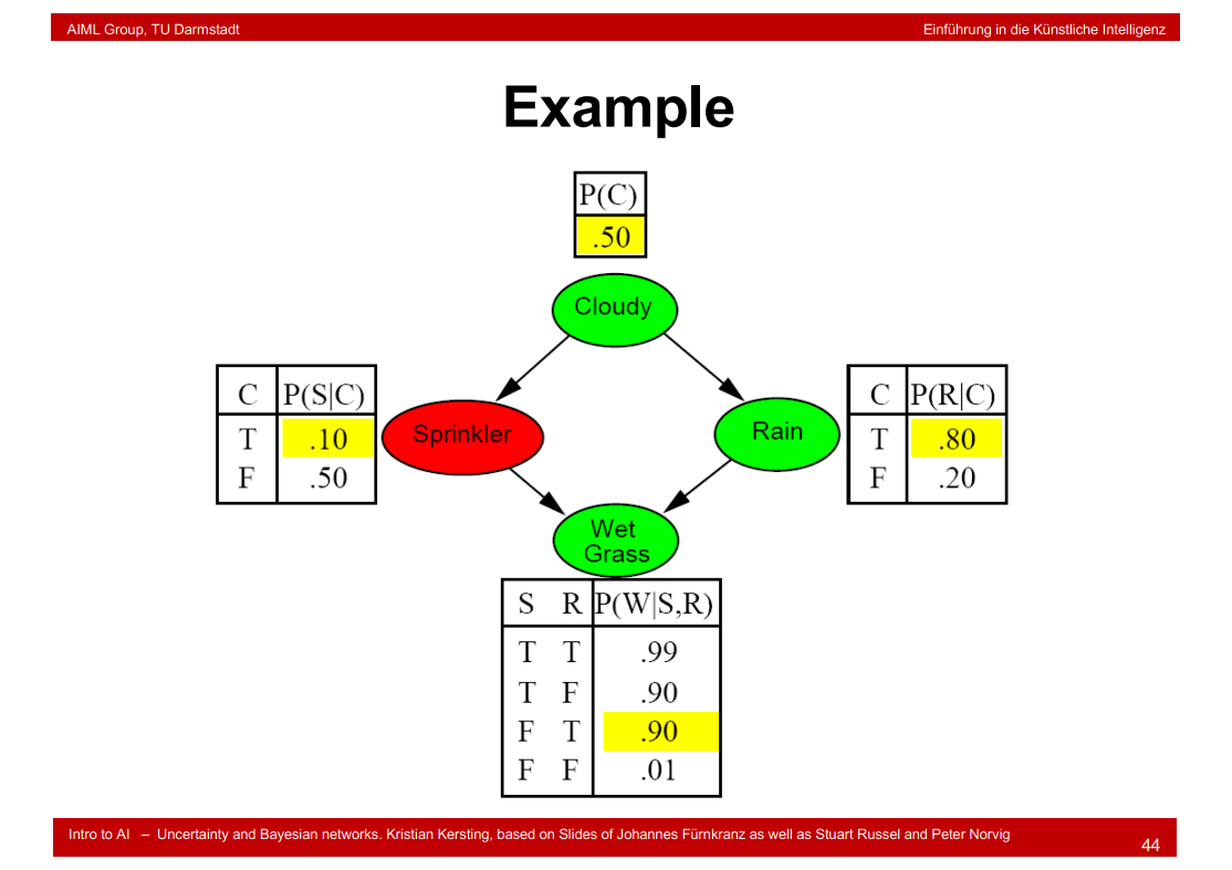
9.17 A very simple example
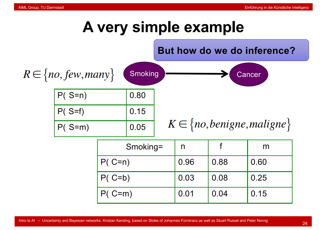
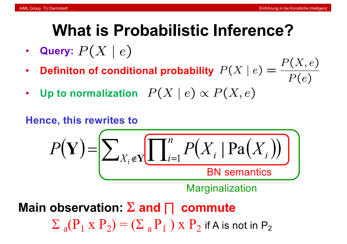
9.18 What is Probabilistic Inference?
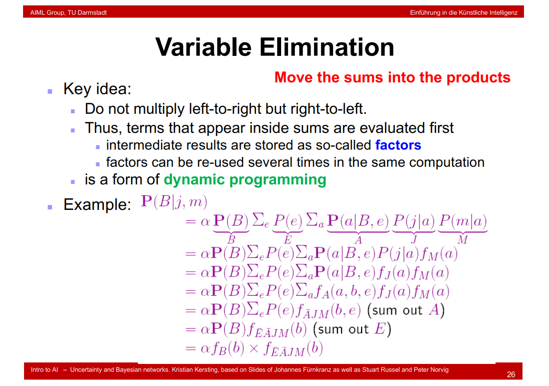
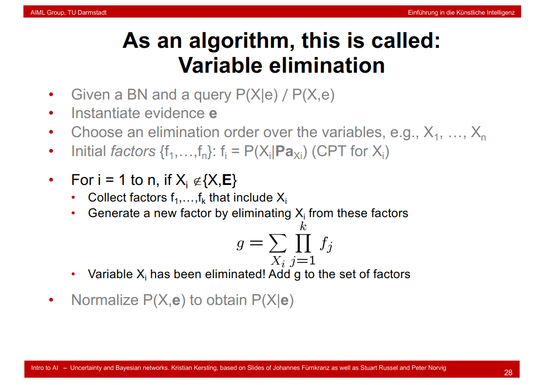
9.19 Variable Elimination
9.20 Complete example: Let’s comput P(L)
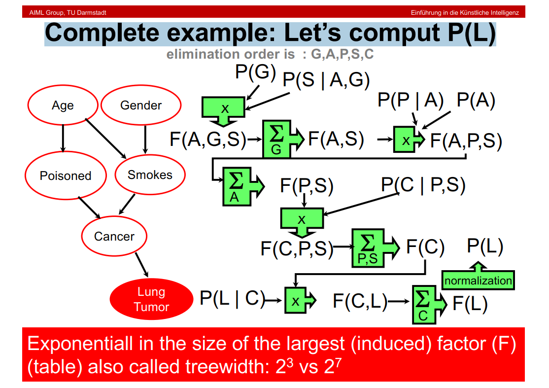
计算过程解释???\(2^{3}\) vs \(2^{7}\)怎么来的??
9.21 As an algorithm, this is called: Variable elimination
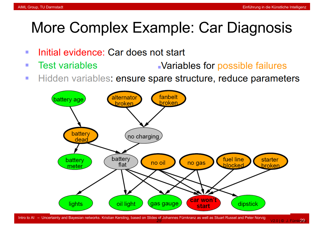
9.22 More Complex Example: Car Diagnosis
9.23 What have we learned so far?
9.24 Mission Completed? No …

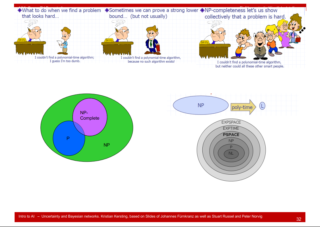
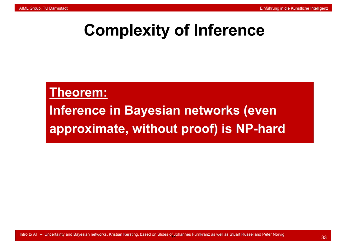
9.25 Complexity of Inference
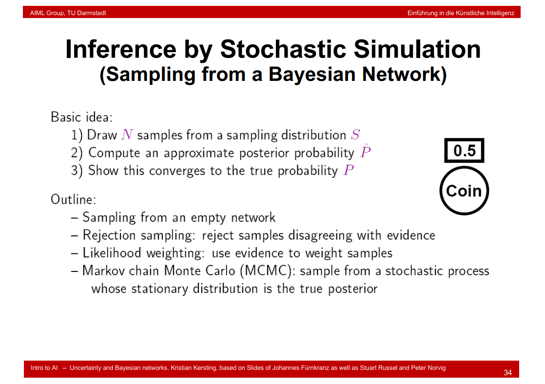
9.26 Inference by Stochastic Simulation (Sampling from a Bayesian Network)
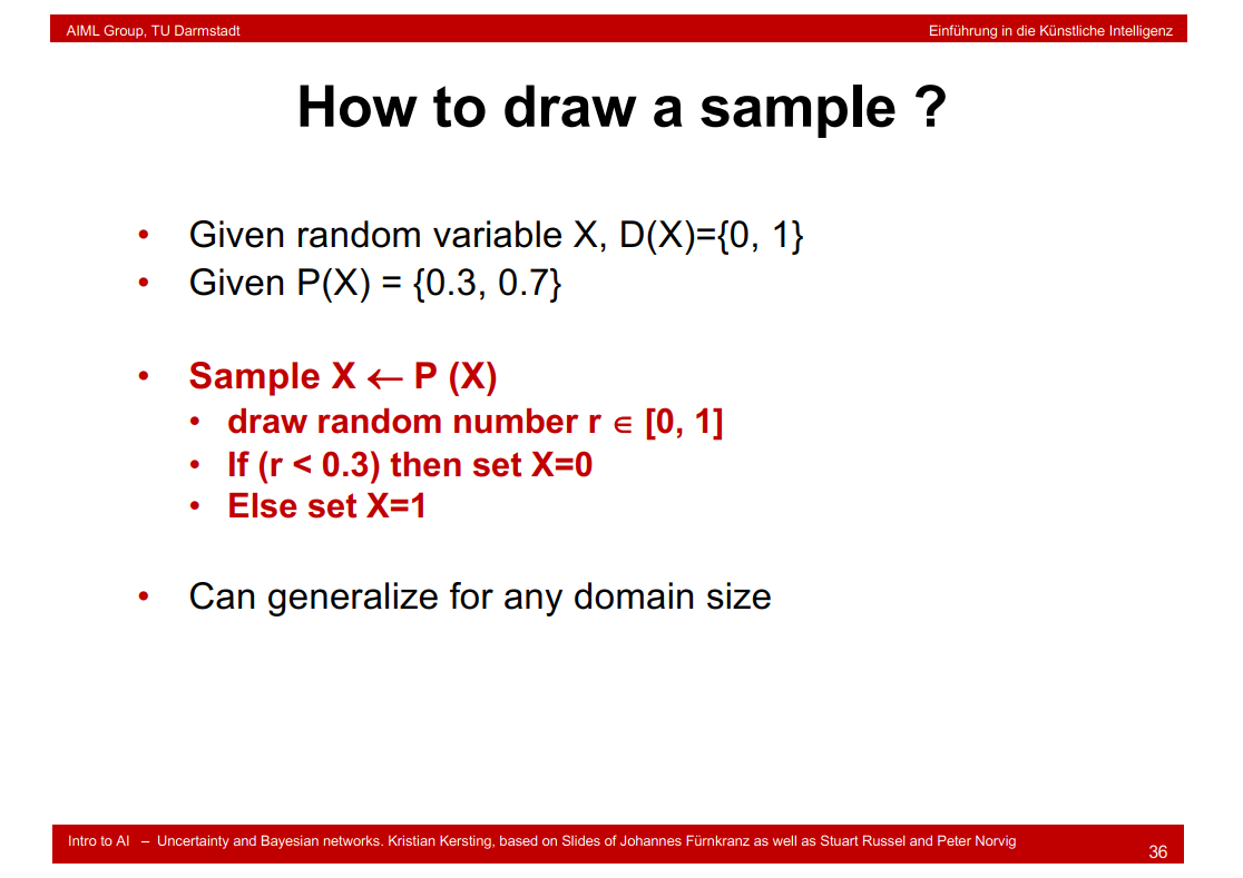
9.27 How to draw a sample ?
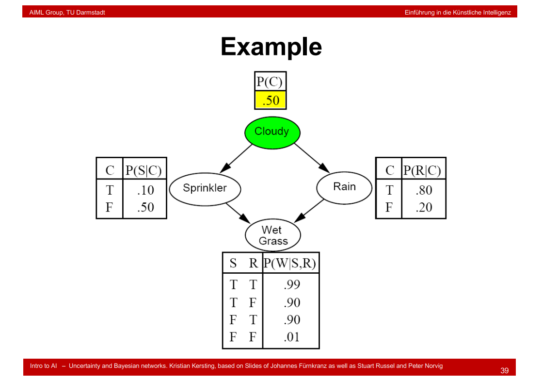
9.28 Example

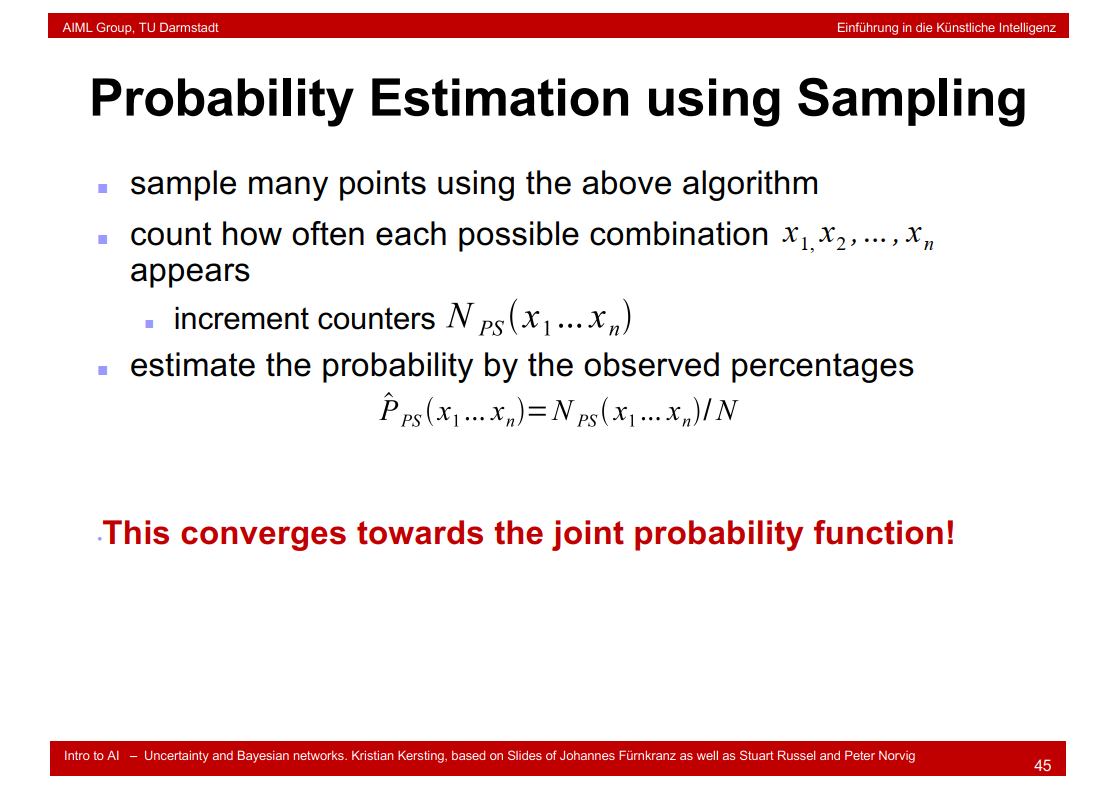
9.29 Probability Estimation using Sampling
9.30 (Directed) Markov Blanket

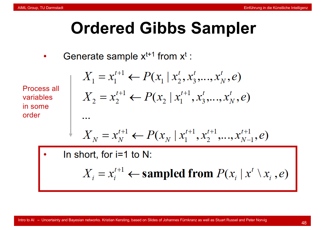
9.31 Ordered Gibbs Sampler
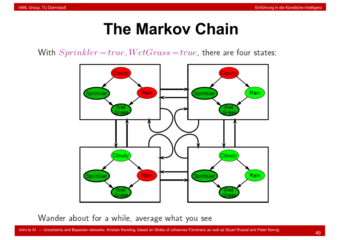
9.32 The Markov Chain
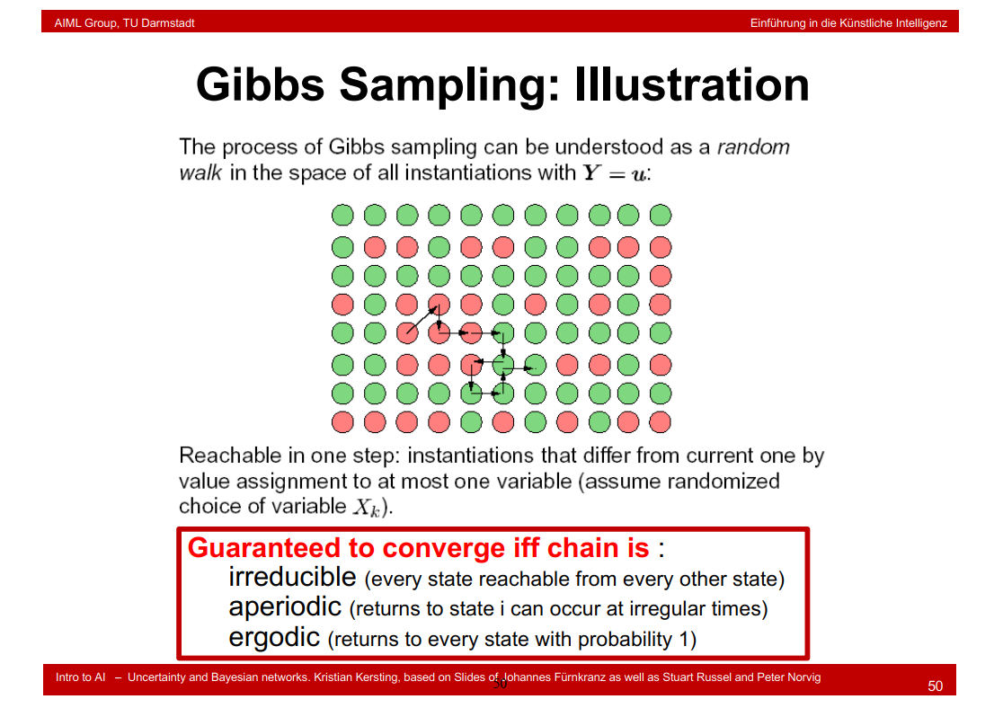
9.33 Gibbs Sampling: Illustration
9.34 Example

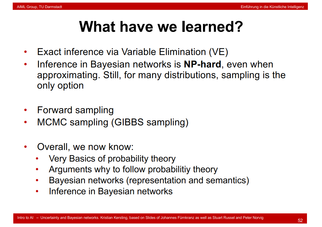
9.35 What have we learned?
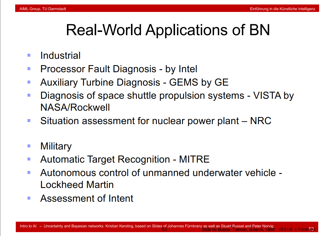
9.36 Real-World Applications of BN

作者:Rest探路者
出处:http://www.cnblogs.com/Java-Starter/
本文版权归作者和博客园共有,欢迎转载,但未经作者同意请保留此段声明,请在文章页面明显位置给出原文连接
Github:https://github.com/cjy513203427

 浙公网安备 33010602011771号