deeplearning----多层感知器
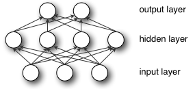
模型:

隐含层激活函数常用的有 或
或 ,由于tanh收敛更快,本文采用tanh函数激活函数。
输出采用逻辑回归G
从逻辑回归到MLP
class HiddenLayer(object):
    def __init__(self, rng, input, n_in, n_out, activation=T.tanh):
        """
        Typical hidden layer of a MLP: units are fully-connected and have
        sigmoidal activation function. Weight matrix W is of shape (n_in,n_out)
        and the bias vector b is of shape (n_out,).

        NOTE : The nonlinearity used here is tanh

        Hidden unit activation is given by: tanh(dot(input,W) + b)

        :type rng: numpy.random.RandomState
        :param rng: a random number generator used to initialize weights

        :type input: theano.tensor.dmatrix
        :param input: a symbolic tensor of shape (n_examples, n_in)

        :type n_in: int
        :param n_in: dimensionality of input

        :type n_out: int
        :param n_out: number of hidden units

        :type activation: theano.Op or function
        :param activation: Non linearity to be applied in the hidden
                              layer
        """
        self.input = input
初始化过程:
# `W` is initialized with `W_values` which is uniformely sampled
# from sqrt(-6./(n_in+n_hidden)) and sqrt(6./(n_in+n_hidden))
# for tanh activation function
# the output of uniform is converted using asarray to dtype
# theano.config.floatX so that the code is runable on GPU
# Note : optimal initialization of weights is dependent on the
#        activation function used (among other things).
#        For example, results presented in [Xavier10]_ suggest that you
#        should use 4 times larger initial weights for sigmoid
#        compared to tanh
#        We have no info for other function, so we use the same as tanh.
W_values = numpy.asarray(rng.uniform(
        low=-numpy.sqrt(6. / (n_in + n_out)),
        high=numpy.sqrt(6. / (n_in + n_out)),
        size=(n_in, n_out)), dtype=theano.config.floatX)
if activation == theano.tensor.nnet.sigmoid:
    W_values *= 4

self.W = theano.shared(value=W_values, name='W')

b_values = numpy.zeros((n_out,), dtype=theano.config.floatX)
self.b = theano.shared(value=b_values, name='b')
所以一个MLP的简单实现如下:
class MLP(object):
  """Multi-Layer Perceptron Class

  A multilayer perceptron is a feedforward artificial neural network model
  that has one layer or more of hidden units and nonlinear activations.
  Intermediate layers usually have as activation function tanh or the
  sigmoid function (defined here by a ``HiddenLayer`` class)  while the
  top layer is a softamx layer (defined here by a ``LogisticRegression``
  class).
  """

  def __init__(self, rng, input, n_in, n_hidden, n_out):
      """Initialize the parameters for the multilayer perceptron

      :type rng: numpy.random.RandomState
      :param rng: a random number generator used to initialize weights

      :type input: theano.tensor.TensorType
      :param input: symbolic variable that describes the input of the
      architecture (one minibatch)

      :type n_in: int
      :param n_in: number of input units, the dimension of the space in
      which the datapoints lie

      :type n_hidden: int
      :param n_hidden: number of hidden units

      :type n_out: int
      :param n_out: number of output units, the dimension of the space in
      which the labels lie

      """

      # Since we are dealing with a one hidden layer MLP, this will
      # translate into a Hidden Layer connected to the LogisticRegression
      # layer
      self.hiddenLayer = HiddenLayer(rng = rng, input = input,
                               n_in = n_in, n_out = n_hidden,
                               activation = T.tanh)

      # The logistic regression layer gets as input the hidden units
      # of the hidden layer
      self.logRegressionLayer = LogisticRegression(
                                  input=self.hiddenLayer.output,
                                  n_in=n_hidden,
                                  n_out=n_out)
同样采用L正则化:
# L1 norm ; one regularization option is to enforce L1 norm to
# be small
self.L1 = abs(self.hiddenLayer.W).sum() \
        + abs(self.logRegressionLayer.W).sum()

# square of L2 norm ; one regularization option is to enforce
# square of L2 norm to be small
self.L2_sqr = (self.hiddenLayer.W ** 2).sum() \
            + (self.logRegressionLayer.W ** 2).sum()

# negative log likelihood of the MLP is given by the negative
# log likelihood of the output of the model, computed in the
# logistic regression layer
self.negative_log_likelihood = self.logRegressionLayer.negative_log_likelihood
# same holds for the function computing the number of errors
self.errors = self.logRegressionLayer.errors

# the parameters of the model are the parameters of the two layer it is
# made out of
self.params = self.hiddenLayer.params + self.logRegressionLayer.params
和之前一样,我们用在mini-batch上面的随机梯度下降算法训练模型。这里的区别在于,我们修改损失函数并包括规范化项。 L1_reg 和 L2_reg 为超参数,用以控制规范化项在整个损失函数中的比重。计算损失的函数如下:
# the cost we minimize during training is the negative log likelihood of
# the model plus the regularization terms (L1 and L2); cost is expressed
# here symbolically
cost = classifier.negative_log_likelihood(y) \
     + L1_reg * L1 \
     + L2_reg * L2_sqr
接下来,模型参数通过梯度更新。这段代码和之前的基本上一样,除了参数多少的差别。
# compute the gradient of cost with respect to theta (stored in params)
# the resulting gradients will be stored in a list gparams
gparams = []
for param in classifier.params:
    gparam  = T.grad(cost, param)
    gparams.append(gparam)


# specify how to update the parameters of the model as a list of
# (variable, update expression) pairs
updates = []
# given two list the zip A = [a1, a2, a3, a4] and B = [b1, b2, b3, b4] of
# same length, zip generates a list C of same size, where each element
# is a pair formed from the two lists :
#    C = [(a1, b1), (a2, b2), (a3, b3) , (a4, b4)]
for param, gparam in zip(classifier.params, gparams):
    updates.append((param, param - learning_rate * gparam))


# compiling a Theano function `train_model` that returns the cost, butx
# in the same time updates the parameter of the model based on the rules
# defined in `updates`
train_model = theano.function(inputs=[index], outputs=cost,
        updates=updates,
        givens={
            x: train_set_x[index * batch_size:(index + 1) * batch_size],
            y: train_set_y[index * batch_size:(index + 1) * batch_size]})
综合所有代码
"""
This tutorial introduces the multilayer perceptron using Theano.

 A multilayer perceptron is a logistic regressor where
instead of feeding the input to the logistic regression you insert a
intermediate layer, called the hidden layer, that has a nonlinear
activation function (usually tanh or sigmoid) . One can use many such
hidden layers making the architecture deep. The tutorial will also tackle
the problem of MNIST digit classification.

.. math::

    f(x) = G( b^{(2)} + W^{(2)}( s( b^{(1)} + W^{(1)} x))),

References:

    - textbooks: "Pattern Recognition and Machine Learning" -
                 Christopher M. Bishop, section 5

"""
__docformat__ = 'restructedtext en'


import cPickle
import gzip
import os
import sys
import time

import numpy

import theano
import theano.tensor as T


from logistic_sgd import LogisticRegression, load_data


class HiddenLayer(object):
    def __init__(self, rng, input, n_in, n_out, W=None, b=None,
                 activation=T.tanh):
        """
        Typical hidden layer of a MLP: units are fully-connected and have
        sigmoidal activation function. Weight matrix W is of shape (n_in,n_out)
        and the bias vector b is of shape (n_out,).

        NOTE : The nonlinearity used here is tanh

        Hidden unit activation is given by: tanh(dot(input,W) + b)

        :type rng: numpy.random.RandomState
        :param rng: a random number generator used to initialize weights

        :type input: theano.tensor.dmatrix
        :param input: a symbolic tensor of shape (n_examples, n_in)

        :type n_in: int
        :param n_in: dimensionality of input

        :type n_out: int
        :param n_out: number of hidden units

        :type activation: theano.Op or function
        :param activation: Non linearity to be applied in the hidden
                           layer
        """
        self.input = input

        # `W` is initialized with `W_values` which is uniformely sampled
        # from sqrt(-6./(n_in+n_hidden)) and sqrt(6./(n_in+n_hidden))
        # for tanh activation function
        # the output of uniform if converted using asarray to dtype
        # theano.config.floatX so that the code is runable on GPU
        # Note : optimal initialization of weights is dependent on the
        #        activation function used (among other things).
        #        For example, results presented in [Xavier10] suggest that you
        #        should use 4 times larger initial weights for sigmoid
        #        compared to tanh
        #        We have no info for other function, so we use the same as
        #        tanh.
        if W is None:
            W_values = numpy.asarray(rng.uniform(
                    low=-numpy.sqrt(6. / (n_in + n_out)),
                    high=numpy.sqrt(6. / (n_in + n_out)),
                    size=(n_in, n_out)), dtype=theano.config.floatX)
            if activation == theano.tensor.nnet.sigmoid:
                W_values *= 4

            W = theano.shared(value=W_values, name='W', borrow=True)

        if b is None:
            b_values = numpy.zeros((n_out,), dtype=theano.config.floatX)
            b = theano.shared(value=b_values, name='b', borrow=True)

        self.W = W
        self.b = b

        lin_output = T.dot(input, self.W) + self.b
        self.output = (lin_output if activation is None
                       else activation(lin_output))
        # parameters of the model
        self.params = [self.W, self.b]


class MLP(object):
    """Multi-Layer Perceptron Class

    A multilayer perceptron is a feedforward artificial neural network model
    that has one layer or more of hidden units and nonlinear activations.
    Intermediate layers usually have as activation function thanh or the
    sigmoid function (defined here by a ``SigmoidalLayer`` class)  while the
    top layer is a softamx layer (defined here by a ``LogisticRegression``
    class).
    """

    def __init__(self, rng, input, n_in, n_hidden, n_out):
        """Initialize the parameters for the multilayer perceptron

        :type rng: numpy.random.RandomState
        :param rng: a random number generator used to initialize weights

        :type input: theano.tensor.TensorType
        :param input: symbolic variable that describes the input of the
        architecture (one minibatch)

        :type n_in: int
        :param n_in: number of input units, the dimension of the space in
        which the datapoints lie

        :type n_hidden: int
        :param n_hidden: number of hidden units

        :type n_out: int
        :param n_out: number of output units, the dimension of the space in
        which the labels lie

        """

        # Since we are dealing with a one hidden layer MLP, this will
        # translate into a TanhLayer connected to the LogisticRegression
        # layer; this can be replaced by a SigmoidalLayer, or a layer
        # implementing any other nonlinearity
        self.hiddenLayer = HiddenLayer(rng=rng, input=input,
                                       n_in=n_in, n_out=n_hidden,
                                       activation=T.tanh)

        # The logistic regression layer gets as input the hidden units
        # of the hidden layer
        self.logRegressionLayer = LogisticRegression(
            input=self.hiddenLayer.output,
            n_in=n_hidden,
            n_out=n_out)

        # L1 norm ; one regularization option is to enforce L1 norm to
        # be small
        self.L1 = abs(self.hiddenLayer.W).sum() \
                + abs(self.logRegressionLayer.W).sum()

        # square of L2 norm ; one regularization option is to enforce
        # square of L2 norm to be small
        self.L2_sqr = (self.hiddenLayer.W ** 2).sum() \
                    + (self.logRegressionLayer.W ** 2).sum()

        # negative log likelihood of the MLP is given by the negative
        # log likelihood of the output of the model, computed in the
        # logistic regression layer
        self.negative_log_likelihood = self.logRegressionLayer.negative_log_likelihood
        # same holds for the function computing the number of errors
        self.errors = self.logRegressionLayer.errors

        # the parameters of the model are the parameters of the two layer it is
        # made out of
        self.params = self.hiddenLayer.params + self.logRegressionLayer.params


def test_mlp(learning_rate=0.01, L1_reg=0.00, L2_reg=0.0001, n_epochs=1000,
             dataset='../data/mnist.pkl.gz', batch_size=20, n_hidden=500):
    """
    Demonstrate stochastic gradient descent optimization for a multilayer
    perceptron

    This is demonstrated on MNIST.

    :type learning_rate: float
    :param learning_rate: learning rate used (factor for the stochastic
    gradient

    :type L1_reg: float
    :param L1_reg: L1-norm's weight when added to the cost (see
    regularization)

    :type L2_reg: float
    :param L2_reg: L2-norm's weight when added to the cost (see
    regularization)

    :type n_epochs: int
    :param n_epochs: maximal number of epochs to run the optimizer

    :type dataset: string
    :param dataset: the path of the MNIST dataset file from
                 http://www.iro.umontreal.ca/~lisa/deep/data/mnist/mnist.pkl.gz


   """
    datasets = load_data(dataset)

    train_set_x, train_set_y = datasets[0]
    valid_set_x, valid_set_y = datasets[1]
    test_set_x, test_set_y = datasets[2]

    # compute number of minibatches for training, validation and testing
    n_train_batches = train_set_x.get_value(borrow=True).shape[0] / batch_size
    n_valid_batches = valid_set_x.get_value(borrow=True).shape[0] / batch_size
    n_test_batches = test_set_x.get_value(borrow=True).shape[0] / batch_size

    ######################
    # BUILD ACTUAL MODEL #
    ######################
    print '... building the model'

    # allocate symbolic variables for the data
    index = T.lscalar()  # index to a [mini]batch
    x = T.matrix('x')  # the data is presented as rasterized images
    y = T.ivector('y')  # the labels are presented as 1D vector of
                        # [int] labels

    rng = numpy.random.RandomState(1234)

    # construct the MLP class
    classifier = MLP(rng=rng, input=x, n_in=28 * 28,
                     n_hidden=n_hidden, n_out=10)

    # the cost we minimize during training is the negative log likelihood of
    # the model plus the regularization terms (L1 and L2); cost is expressed
    # here symbolically
    cost = classifier.negative_log_likelihood(y) \
         + L1_reg * classifier.L1 \
         + L2_reg * classifier.L2_sqr

    # compiling a Theano function that computes the mistakes that are made
    # by the model on a minibatch
    test_model = theano.function(inputs=[index],
            outputs=classifier.errors(y),
            givens={
                x: test_set_x[index * batch_size:(index + 1) * batch_size],
                y: test_set_y[index * batch_size:(index + 1) * batch_size]})

    validate_model = theano.function(inputs=[index],
            outputs=classifier.errors(y),
            givens={
                x: valid_set_x[index * batch_size:(index + 1) * batch_size],
                y: valid_set_y[index * batch_size:(index + 1) * batch_size]})

    # compute the gradient of cost with respect to theta (sotred in params)
    # the resulting gradients will be stored in a list gparams
    gparams = []
    for param in classifier.params:
        gparam = T.grad(cost, param)
        gparams.append(gparam)

    # specify how to update the parameters of the model as a list of
    # (variable, update expression) pairs
    updates = []
    # given two list the zip A = [a1, a2, a3, a4] and B = [b1, b2, b3, b4] of
    # same length, zip generates a list C of same size, where each element
    # is a pair formed from the two lists :
    #    C = [(a1, b1), (a2, b2), (a3, b3), (a4, b4)]
    for param, gparam in zip(classifier.params, gparams):
        updates.append((param, param - learning_rate * gparam))

    # compiling a Theano function `train_model` that returns the cost, but
    # in the same time updates the parameter of the model based on the rules
    # defined in `updates`
    train_model = theano.function(inputs=[index], outputs=cost,
            updates=updates,
            givens={
                x: train_set_x[index * batch_size:(index + 1) * batch_size],
                y: train_set_y[index * batch_size:(index + 1) * batch_size]})

    ###############
    # TRAIN MODEL #
    ###############
    print '... training'

    # early-stopping parameters
    patience = 10000  # look as this many examples regardless
    patience_increase = 2  # wait this much longer when a new best is
                           # found
    improvement_threshold = 0.995  # a relative improvement of this much is
                                   # considered significant
    validation_frequency = min(n_train_batches, patience / 2)
                                  # go through this many
                                  # minibatche before checking the network
                                  # on the validation set; in this case we
                                  # check every epoch

    best_params = None
    best_validation_loss = numpy.inf
    best_iter = 0
    test_score = 0.
    start_time = time.clock()

    epoch = 0
    done_looping = False

    while (epoch < n_epochs) and (not done_looping):
        epoch = epoch + 1
        for minibatch_index in xrange(n_train_batches):

            minibatch_avg_cost = train_model(minibatch_index)
            # iteration number
            iter = (epoch - 1) * n_train_batches + minibatch_index

            if (iter + 1) % validation_frequency == 0:
                # compute zero-one loss on validation set
                validation_losses = [validate_model(i) for i
                                     in xrange(n_valid_batches)]
                this_validation_loss = numpy.mean(validation_losses)

                print('epoch %i, minibatch %i/%i, validation error %f %%' %
                     (epoch, minibatch_index + 1, n_train_batches,
                      this_validation_loss * 100.))

                # if we got the best validation score until now
                if this_validation_loss < best_validation_loss:
                    #improve patience if loss improvement is good enough
                    if this_validation_loss < best_validation_loss *  \
                           improvement_threshold:
                        patience = max(patience, iter * patience_increase)

                    best_validation_loss = this_validation_loss
                    best_iter = iter

                    # test it on the test set
                    test_losses = [test_model(i) for i
                                   in xrange(n_test_batches)]
                    test_score = numpy.mean(test_losses)

                    print(('     epoch %i, minibatch %i/%i, test error of '
                           'best model %f %%') %
                          (epoch, minibatch_index + 1, n_train_batches,
                           test_score * 100.))

            if patience <= iter:
                    done_looping = True
                    break

    end_time = time.clock()
    print(('Optimization complete. Best validation score of %f %% '
           'obtained at iteration %i, with test performance %f %%') %
          (best_validation_loss * 100., best_iter + 1, test_score * 100.))
    print >> sys.stderr, ('The code for file ' +
                          os.path.split(__file__)[1] +
                          ' ran for %.2fm' % ((end_time - start_time) / 60.))


if __name__ == '__main__':
    test_mlp()

 浙公网安备 33010602011771号