Datawhale 组队学习 🐋fun-transformer Task 05 🐆项目案例

Datawhale 组队学习 fun-transformer

Task 5 项目案例

Datawhale项目链接：https://www.datawhale.cn/learn/summary/87

笔记作者：博客园-岁月月宝贝💫

微信名：有你在就不需要🔮给的勇气

目录

• Datawhale 组队学习 fun-transformer
  • 💐使用 NumPy 和 SciPy 实现通用注意力机制
    • 1.定义词向量
    • 2.生成权重矩阵
    • 3.计算查询、键和值
    • 4.计算得分
    • 5.计算权重
    • 6.计算注意力输出
  • 💐自注意力机制
    • 1.定义输入序列
    • 2.生成权重矩阵
    • 3.计算 Key、Query 和 Value 矩阵
    • 4.计算注意力分数
    • 5.计算注意力权重
    • 6.计算注意力输出
  • 💐多头注意力机制
    • 1.MultiHeadAttention 类
    • 2.主函数
  • 💐Transformer组件实现
    • 1.必导库
    • 2.位置编码
    • 3.多头注意力
    • 4.前馈网络
    • 5.编码器
    • 6.解码器
    • 7.Transformer模型
    • 8.Transformer模型的训练和评估
  • 💐实践项目
    • 1.库的准备
    • 2.数据准备
    • 3.数据加载
    • 4.位置编码
    • 5.Mask使用->多头自注意力机制
    • 6.前馈神经网络
    • 7.编码器和解码器
      • 🌷1. 模型的整体结构
        • 1.1 编码器 (Encoder)
        • 1.2 解码器 (Decoder)
      • 🌷2.Encoder Layer (编码器层)
      • 🌷3.Encoder (编码器)
      • 🌷4.Decoder Layer(解码器层)
      • 🌷5.Decoder(解码器)
    • 8.Transformer模型
    • 9.训练和测试
      • 🐮1.定义模型、损失函数和优化器
      • 🐮2.训练模型
      • 🐮3.测试模型
      • 🐮4.测试示例

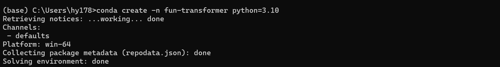
准备工作

因为我的电脑是GPU版的，之前的深度学习环境不小心因为“大小写不敏感”的重名环境影响而误删了，这节就带大家一起手把手小小创建环境安装GPU版的torch&它的朋友们💪

电脑版本：win11

1.点击屏幕右下角这个小绿色按钮

2.查看电脑显卡驱动版本

点击“系统信息”-点击“组件”

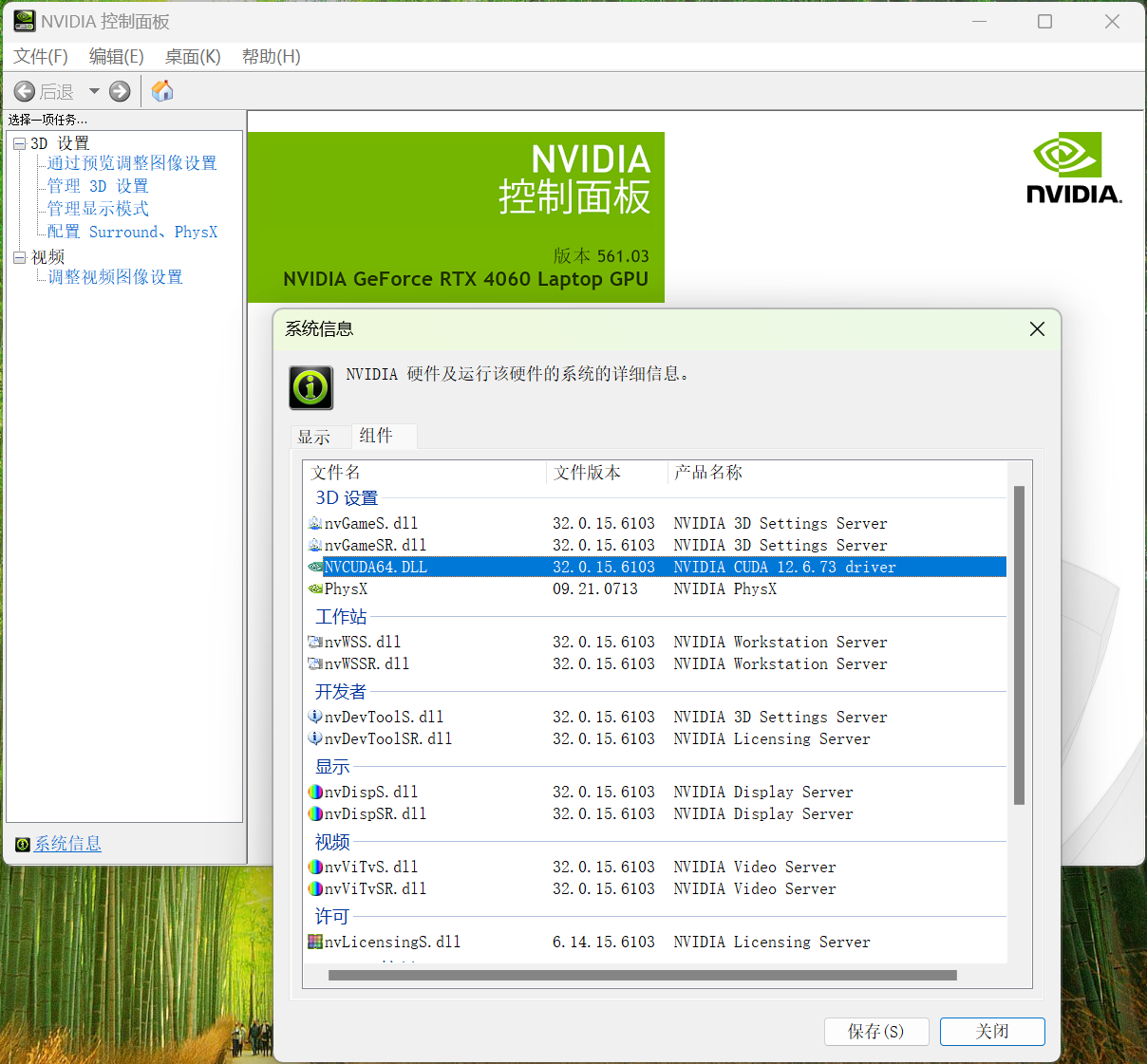
可以发现版本为12.6

3.进入pytorch官网 https://pytorch.org/

由于我的显卡版本是12.6，只要安装小于等于12.6的Compute Platform均可以~

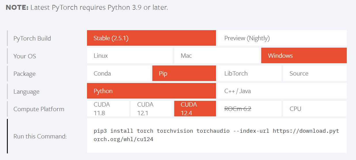
pip3 install torch torchvision torchaudio --index-url https://download.pytorch.org/whl/cu124

4.下面，我们开始配python环境

🌟首先注意，Python版本不能低于3.9哦~

so,我又选了喜欢的python3.10

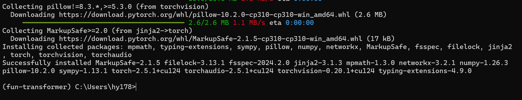
激活环境，开始安装！

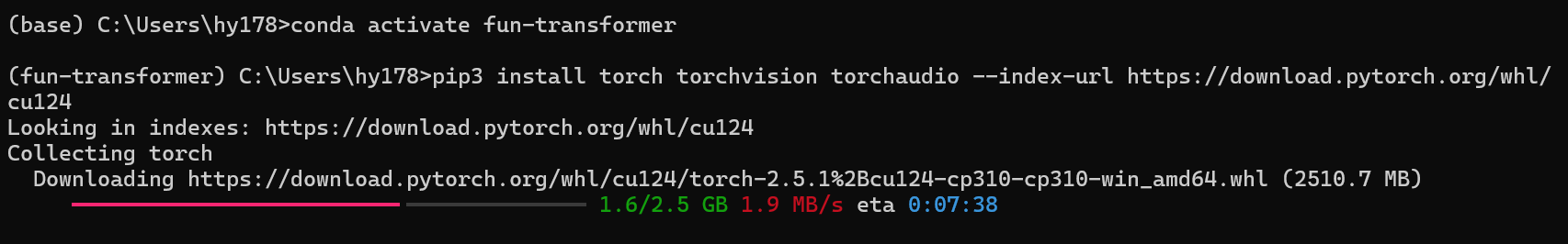
安装成功！

😊如果大家还有问题，可以看这个链接喵：全网最详细的安装pytorch GPU方法，一次安装成功！！包括安装失败后的处理方法！-CSDN博客

（今天有点开心喵，通过Datawhale冬令营第二期荣获豆包Marscode MVP荣誉😝，可以说努力就有回报！大家也加油！！！）

实践部分

实践理论除了DW教程还可能会参照：

• 手撕Transformer！！从每一模块原理讲解到代码实现【超详细！】_手撕 transformer-CSDN博客
• zxuu/Self-Attention: Transformer的完整实现。详细构建Encoder、Decoder、Self-attention。以实际例子进行展示，有完整的输入、训练、预测过程。可用于学习理解self-attention和Transformer
• 【手撕Transformer】Transformer输入输出细节以及代码实现（pytorch）_51CTO博客_transformer的输入输出

芜湖！学习列车开始啦！★,°:.☆(￣▽￣)/$:.°★ 。

💐使用 NumPy 和 SciPy 实现通用注意力机制

1.定义词向量

import numpy as np
from scipy.special import softmax

# 首先，我们定义四个单词的词向量，每个向量维度为3。
word_1 = np.array([1, 0, 0])
word_2 = np.array([0, 1, 0])
word_3 = np.array([1, 1, 0])
word_4 = np.array([0, 0, 1])
words = np.array([word_1, word_2, word_3, word_4])

words（4行3列）：

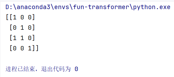
单词堆叠形成的矩阵，其中每一行代表一个单词的收入。

word_x:维度1*3，代表一个单词在嵌入空间中的表示。

2.生成权重矩阵

接下来，我们生成三个权重矩阵\(W_Q\), \(W_K\), \(W_V\)

# 生成权重矩阵
np.random.seed(42) # 设置随机数种子，确保每次运行代码时生成的权重矩阵相同。
W_Q = np.random.randint(3, size=(3, 3))
W_K = np.random.randint(3, size=(3, 3))
W_V = np.random.randint(3, size=(3, 3))

我们的三个权重矩阵(维度均为3*3)：

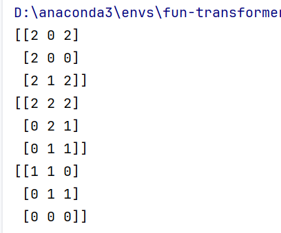
这些权重矩阵用于将词向量转换为查询（Query）、键（Key）和值（Value）。

3.计算查询、键和值

🌟将输入词向量与权重矩阵相乘，得到查询、键和值。

# generating the queries, keys and values
Q = words @ W_Q
K = words @ W_K
V = words @ W_V

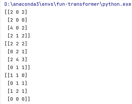
我们的查询Q、键K与值V（维度均为4*3）：

4.计算得分

🌟得分矩阵score通过查询矩阵Q和键矩阵K的转置矩阵乘法得到。

# scoring the query vectors against all key vectors
scores = Q @ K.T

我们的scores矩阵（维度4*4）

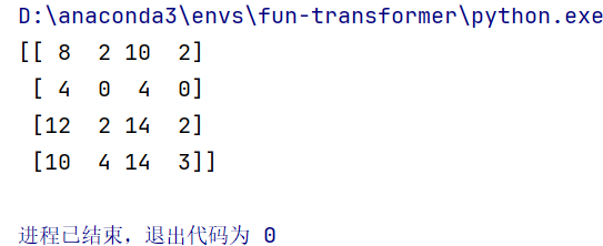
数学上，这可以表示为： \(\mathrm{scores}=Q\cdot K^T\in\mathbb{R}^{4\times4}\)

其中 \(scores_{ij}\) 表示第 i 个查询向量 \(Q_i\) 与第 j 个键向量 \(K_j\) 的相似度，计算方式为点积：

\(\mathrm{scores}_{ij}=Q_i\cdot K_j=\sum_{k=1}^3Q_{ik}K_{jk}\)

5.计算权重

🌟使用softmax函数将得分转换为概率分布，得到注意力权重。

# computing the weights by a softmax operation
weights = softmax(scores / np.sqrt(K.shape[1]), axis=1)

K.shape[1]:是K一行的元素数目，我们这里对应3。

scores / np.sqrt(K.shape[1]):对得分scores进行缩放，保持数值稳定性，缩放后scores维度依然是4*4。

axis=1:表示沿着矩阵的行进行softmax处理。softmax会将缩放后的scores矩阵每行的每个元素变成\(e^{这个元素}\) / 这行所有元素的\(e^{每个元素}\)的和,所以weighs维度等于缩放后的scores矩阵的维度，所以也等于得分scores矩阵的维度。

数学公式：

softmax函数：\(\mathrm{softmax}(x)_i=\frac{e^{x_i}}{\sum_je^{x_j}}\)

缩放后的scores矩阵：\(\text{scaled scores}=\frac{\mathrm{scores}}{\sqrt{K.shape[1]}}\)

weights矩阵里的每个元素：\(\mathrm{weights}_{ij}=\frac{e^{{\mathrm{scaled scores}_{ij}}}}{\sum_{k=1}^{4}e^{{\mathrm{scaled scores}_{ik}}}}\)

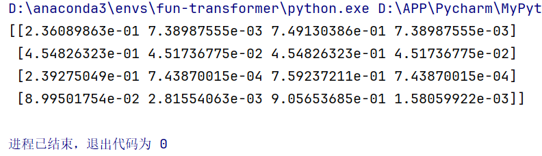
weights矩阵：

6.计算注意力输出

🌟最后，我们通过加权和(注意力权重与值矩阵相乘)的方式计算注意力输出。

# computing the attention by a weighted sum of the value vectors
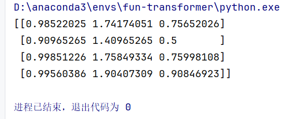
attention = weights @ V

print(attention)

attention矩阵：

数学上，这可以表示为：\(\text{attention}=\mathrm{weights}\cdot V\in\mathbb{R}^{4\times3}\)

4×4的矩阵与4×3的矩阵相乘，获得4×4的矩阵

其中，每个元素 \(attention_i\) (attention矩阵i那行)是所有值(列)向量（针对第i行权重）的加权和：

\(\text{attention}_i=\sum_{j=1}^4\mathrm{weights}_{ij}V_j\)

这样，我们得到了每个输入位置的注意力输出，它综合了输入序列中所有单词的信息，其中每个单词的贡献程度由注意力权重决定。

这个数学推理过程展示了注意力机制如何通过动态地计算权重来聚焦于输入序列中最相关的部分，从而生成更准确的输出。

💐自注意力机制

1.定义输入序列

# 导入库
import torch
import torch.nn.functional as F

# 示例输入序列
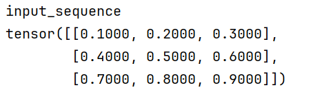
input_sequence = torch.tensor([[0.1, 0.2, 0.3], [0.4, 0.5, 0.6], [0.7, 0.8, 0.9]])

print("input_sequence")
print(input_sequence)

输出为3*3的矩阵

2.生成权重矩阵

# 生成 Key、Query 和 Value 矩阵的随机权重
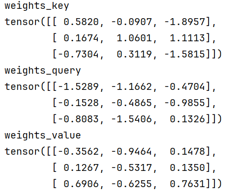
random_weights_key = torch.randn(input_sequence.size(-1), input_sequence.size(-1))
random_weights_query = torch.randn(input_sequence.size(-1), input_sequence.size(-1))
random_weights_value = torch.randn(input_sequence.size(-1), input_sequence.size(-1))

print("weights_key")
print(random_weights_key)
print("weights_query")
print(random_weights_query)
print("weights_value")
print(random_weights_value)

size(-1) 将返回最后一个维度的大小，因为列为3，input_sequence.size(-1)即为3

torch.randn 的参数是张量的形状，最后会生成一个内部元素均服从标准正态分布（均值为 0，标准差为 1）的随机数张量。

输出均为3*3的矩阵

3.计算 Key、Query 和 Value 矩阵

# 计算 Key、Query 和 Value 矩阵
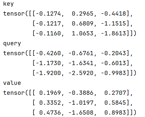
key = torch.matmul(input_sequence, random_weights_key)
query = torch.matmul(input_sequence, random_weights_query)
value = torch.matmul(input_sequence, random_weights_value)

print("key")
print(key)
print("query")
print(query)
print("value")
print(value)

torch.matmul 是 PyTorch 中的矩阵乘法函数，用于计算两个张量的矩阵乘积。对于两个二维张量（矩阵），torch.matmul 的行为与 NumPy 中的 np.dot 类似。

所以，输出均为3*3的矩阵

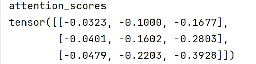
4.计算注意力分数

疑似缩放后的scores矩阵

attention_scores = torch.matmul(query, key.T) / torch.sqrt(torch.tensor(query.size(-1), dtype=torch.float32))

print("attention_scores")
print(attention_scores)

Q:为什么使用 query.size(-1) 而不是 K 的一行元素的个数？

A: 在注意力机制中，query 和 key 通常具有相同的维度，这是因为它们都是从相同的输入序列通过不同的权重矩阵变换得到的。因此，query.size(-1) 和 key.size(-1) 通常是相等的。

在代码中，query 和 key 都是从 input_sequence 通过不同的随机权重矩阵变换得到的，它们的形状都是 (3, 3)。因此，query.size(-1) 和 key.size(-1) 都是 3。

易得，输出均为3*3的矩阵：

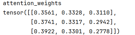
5.计算注意力权重

和前面方法一模一样

# 使用 softmax 函数获得注意力权重("dim=-1"算的是行嘛？)
attention_weights = F.softmax(attention_scores, dim=-1)

print("attention_weights")
print(attention_weights)

Q：dim=-1 的含义？

A：对于一个二维张量（矩阵），dim=-1 表示沿着列进行操作，即对每一行的元素进行 softmax 计算。具体来说，F.softmax(attention_scores, dim=-1) 会对 attention_scores 的每一行进行 softmax 操作，使得每一行的元素之和为 1。

易得，输出为3*3的矩阵

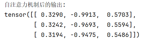
6.计算注意力输出

# 计算 Value 向量的加权和
output = torch.matmul(attention_weights, value)

print("自注意力机制后的输出:")
print(output)

3*3的两个矩阵相乘，得到矩阵：

💐多头注意力机制

1.MultiHeadAttention 类

import math
import torch
import torch.nn as nn
import torch.nn.functional as F

# 定义一个 MultiHeadAttention 类，它继承自 nn.Module---------------------------
class MultiHeadAttention(nn.Module):
    def __init__(self, heads, d_model, dropout=0.1):
        # 调用父类的构造函数
        super().__init__()

        # 保存模型维度和头数
        self.d_model = d_model
        self.d_k = d_model // heads  # 每个头对应的维度(//是整除的意思啦！)
        self.h = heads  # 头的数量

        # 初始化线性层，用于将输入转换为查询（Q）、键（K）和值（V）
        self.q_linear = nn.Linear(d_model, d_model)#这个线性层将输入数据转换为查询（Query），输入维度是 d_model，输出维度也是 d_model。
        self.k_linear = nn.Linear(d_model, d_model)
        self.v_linear = nn.Linear(d_model, d_model)

        # 初始化Dropout层，用于正则化
        self.dropout = nn.Dropout(dropout)

        # 初始化输出线性层，用于将多头注意力输出转换为模型维度
        self.out = nn.Linear(d_model, d_model)

    # 定义注意力机制的计算过程🚪--------------------------------------------
    def attention(self, q, k, v, mask=None):
        # 计算Q和K的矩阵乘积，然后除以根号下d_k
        scores = torch.matmul(q, k.transpose(-2, -1)) / math.sqrt(self.d_k)
        #😘k.transpose(-2, -1) 表示交换张量 k 的倒数第二个维度和最后一个维度。也代表行列互换！
        
        # 如果提供了掩码，则将掩码对应的位置设置为负无穷，这样在softmax后这些位置的值为0
        if mask is not None:
            scores = scores.masked_fill(mask == 0, -1e9)

        # 应用softmax函数获得注意力权重
        scores = F.softmax(scores, dim=-1)

        # 应用dropout
        scores = self.dropout(scores)

        # 将注意力权重和V相乘得到输出
        output = torch.matmul(scores, v)

        return output

    # 定义前向传播过程------------------------------------------------------
    def forward(self, q, k, v, mask=None):
        batch_size = q.size(0)#返回的是q的第一个维度大小

        # 将输入Q、K、V通过线性层，并调整形状以进行多头注意力计算
        q = self.q_linear(q).view(batch_size, -1, self.h, self.d_k).transpose(1, 2)
        k = self.k_linear(k).view(batch_size, -1, self.h, self.d_k).transpose(1, 2)
        v = self.v_linear(v).view(batch_size, -1, self.h, self.d_k).transpose(1, 2)
        
        #view 方法用于改变张量的形状
        # batch_size 是批次大小，表示批次中包含的样本数量。
        # -1 是一个特殊值，表示自动计算该维度的大小，以确保数据的总元素数量不变。
        # self.h 是头的数量。
        # self.d_k 是每个头对应的维度。

        #transpose 方法用于交换张量的两个维度。
        #transpose(1, 2) 交换了第一个维度和第二个维度(从第零个维度开始算)，将张量的形状从 (batch_size, sequence_length, heads, d_k) 变为 (batch_size, heads, sequence_length, d_k)

        # 计算注意力输出(调用了上面注意力机制的计算函数~🚪)
        scores = self.attention(q, k, v, mask)

        # 将多头输出合并，并调整形状以匹配模型维度
        concat = scores.transpose(1, 2).contiguous().view(batch_size, -1, self.d_model)#维度转回，向量合并！！！

        # 通过输出线性层
        output = self.out(concat)

        return output

Q：多头注意力机制中scores = torch.matmul(q, k.transpose(-2, -1)) / math.sqrt(self.d_k)为什么不是像单头注意力机制weights = softmax(scores / np.sqrt(K.shape[1]), axis=1)一样除以根号K？

A：在多头注意力机制中，我们需要对每个头的点积结果进行缩放，而不是对所有头合并后的点积结果进行缩放。这就是为什么我们在多头注意力机制中使用 self.d_k（即每个头的维度）来进行缩放，而不是使用 d_model（即所有头合并后的总维度）。

Q：为什么“concat = scores.transpose(1, 2).contiguous().view(batch_size, -1, self.d_model)”会加入contiguous()?

A: 在 PyTorch 中，.contiguous() 方法用于确保张量在内存中是连续存储的。在 PyTorch 中进行某些操作，比如转置（transpose）、扩展（expand）等，可能会改变张量在内存中的存储顺序，使得张量不再连续。当张量不再连续时，某些操作（比如 .view()）就无法直接进行，因为这些操作要求张量在内存中必须是连续的。

.contiguous() 方法会返回一个新的张量，这个张量在内存中是连续的。它不会修改原始张量，而是返回一个新的视图（view），这个视图在内存中是连续的。

2.主函数

# 主函数，用于测试 MultiHeadAttention 类-------------------------------------
if __name__ == "__main__":
    # 初始化模型参数
    heads = 4
    d_model = 128  # d_model应该是heads的整数倍。
    dropout = 0.1

    # 创建 MultiHeadAttention 实例
    model = MultiHeadAttention(heads, d_model, dropout)#设计者规定

    # 创建随机数据作为输入
    batch_size = 2
    seq_len = 5
    q = torch.rand(batch_size, seq_len, d_model)  # Query
    k = torch.rand(batch_size, seq_len, d_model)  # Key
    v = torch.rand(batch_size, seq_len, d_model)  # Value

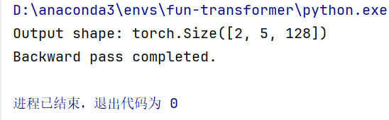
    # 执行前向传播
    output = model(q, k, v)

    # 打印输出形状，应该是 [batch_size, seq_len, d_model]
    print("Output shape:", output.shape)#下面会讲为什么是这样的

    # 检查模型是否可以进行反向传播
    loss = output.mean()  # 创建一个简单的损失函数
    loss.backward()  # 执行反向传播
    print("Backward pass completed.")  # 如果没有错误，则表示反向传播成功

输出展示：

Q: 为什么最终维度一定是`[batch_size, seq_len, d_model]`?

A: 在多头注意力机制中，输出形状 [batch_size, seq_len, d_model] 是由模型的设计和前向传播过程决定的。让我们逐步解析为什么输出形状会是这样。

1. 输入数据的形状

假设输入数据 q、k 和 v 的形状分别是 [batch_size, seq_len, d_model]，其中：

• batch_size 是批次大小，表示批次中包含的样本数量。
• seq_len 是序列长度，表示每个样本中的序列元素数量。
• d_model 是模型的维度，表示每个序列元素的特征数量。
• 例如，我们输入的q、k 和 v 的形状是 [2, 5, 128]，表示有 2 个样本，每个样本有 5 个序列元素，每个元素有 128 个特征。

2. 多头注意力机制的前向传播过程

在多头注意力机制中，输入数据 q、k 和 v 会经过以下步骤：

1. 线性变换:
   • q、k 和 v 分别通过线性层 q_linear、k_linear 和 v_linear，将输入数据转换为查询（Query）、键（Key）和值（Value）。这些线性层的输入和输出维度都是 d_model。
   • 线性变换后的形状仍然是 [batch_size, seq_len, d_model]。
   • 所以，我们q_linear(q)、k_linear(k) 和 v_linear(v) 的输出形状仍然是 [2, 5, 128]。
2. 分头:
   • 将查询（Query）、键（Key）和值（Value）分成多个头。每个头的维度是 d_k = d_model // heads。
   • 分头后的形状变为 [batch_size, seq_len, heads, d_k]。
   • 通过 transpose(1, 2) 将形状调整为 [batch_size, heads, seq_len, d_k]。
   • 我们分头后的q、k、v形状变为 [2, 5, 4, 32]，然后通过 transpose(1, 2) 调整为 [2, 4, 5, 32]。
3. 计算注意力分数:
   • 计算查询（Query）和键（Key）的点积，得到注意力分数。
   • 注意力分数的形状是 [batch_size, heads, seq_len, seq_len]。
   • 所以我们注意力分数的形状是 [2, 4, 5, 5]。
4. 应用 Softmax 和 Dropout:
   • 对注意力分数应用 Softmax 函数，得到注意力权重。
   • 对注意力权重应用 Dropout，防止过拟合。
5. 加权求和:
   • 使用注意力权重对值（Value）进行加权求和，得到每个头的输出。
   • 每个头的输出形状是 [batch_size, heads, seq_len, d_k]。
   • 我们每个头的输出形状是 [2, 4, 5, 32]。
6. 合并头:
   • 将所有头的输出拼接起来，形状变为 [batch_size, seq_len, heads * d_k]。
   • 由于 heads * d_k = d_model，拼接后的形状是 [batch_size, seq_len, d_model]。
   • 我们拼接后的形状是 [2, 5, 128]。
7. 输出线性层:
   • 通过输出线性层 out，将拼接后的输出转换为最终的输出。
   • 最终输出的形状是 [batch_size, seq_len, d_model]。
   • 所以，我们最终输出的形状是 [2, 5, 128]。

总结
🌹输出形状 `[batch_size, seq_len, d_model]` 是由多头注意力机制的设计和前向传播过程决定的。
🌹每个头的输出在合并后会恢复到原始的模型维度 `d_model`，并通过输出线性层进行最终转换。

💐Transformer组件实现

1.必导库

import math
import torch
import torch.nn as nn
import torch.optim as optim
import torch.nn.functional as F

2.位置编码

class PositionalEncoding(nn.Module):
    def __init__(self, d_model, max_len=5000):
        super(PositionalEncoding, self).__init__()

        # 计算位置编码
        pe = torch.zeros(max_len, d_model)#创建一个形状为 `(max_len, d_model)` 的零张量，用于存储位置编码
        position = torch.arange(0, max_len, dtype=torch.float).unsqueeze(1)#创建一个形状为 `(max_len, 1)` 的张量，表示位置索引。
        div_term = torch.exp(torch.arange(0, d_model, 2).float() * (-torch.log(
            torch.tensor(10000.0)) / d_model))#计算分母项，用于调整频率。
        pe[:, 0::2] = torch.sin(position * div_term)#偶数维度的位置编码
        pe[:, 1::2] = torch.cos(position * div_term)#奇数维度的位置编码
        pe = pe.unsqueeze(0)#将位置编码的形状从 `(max_len, d_model)` 调整为 `(1, max_len, d_model)`
        self.register_buffer('pe', pe)#将位置编码注册为模型的缓冲区

    def forward(self, x):
        x = x + self.pe[:, :x.size(1)]#将位置编码添加到输入数据 `x` 中
        return x#返回添加了位置编码的输入数据

# 示例用法
d_model = 512
max_len = 100
num_heads = 8

# 位置编码--------------------------512-------100
pos_encoder = PositionalEncoding(d_model, max_len)

# 示例输入序列--------------------100-------512
input_sequence = torch.randn(5, max_len, d_model)

# 应用位置编码
input_sequence = pos_encoder(input_sequence)
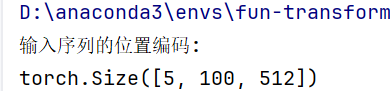
print("输入序列的位置编码:")
print(input_sequence.shape)

难点细讲

1. position = torch.arange(0, max_len, dtype=torch.float).unsqueeze(1):
   • torch.arange(0, max_len, dtype=torch.float) 生成一个从 0 到 max_len-1 的浮点数序列。
   • .unsqueeze(1) 增加一个维度，将形状从 (max_len) 调整为 (max_len, 1)。
2. div_term = torch.exp(torch.arange(0, d_model, 2).float() * (-torch.log(torch.tensor(10000.0)) / d_model)):
   • torch.arange(0, d_model, 2) 生成一个从 0 到 d_model-1 的偶数序列。
   • torch.log(torch.tensor(10000.0)) 计算 10000 的自然对数。torch.tensor(10000.0)：创建一个包含单个元素 10000.0 的 PyTorch 张量。
   • torch.exp(...) 计算 e...。
3. pe[:, 0::2] = torch.sin(position * div_term):
   • 计算偶数维度的位置编码，使用正弦函数。
   • position * div_term 计算位置索引和分母项的乘积。
   • torch.sin(...) 计算正弦值。
4. pe[:, 1::2] = torch.cos(position * div_term):
   • 计算奇数维度的位置编码，使用余弦函数。
   • position * div_term 计算位置索引和分母项的乘积。
   • torch.cos(...) 计算余弦值。
5. pe = pe.unsqueeze(0):
   • .unsqueeze(0) 方法用于在指定的维度上增加一个大小为 1 的新维度，将位置编码的形状从 (max_len, d_model) 调整为 (1, max_len, d_model)，以便与输入数据的批次维度对齐。
6. self.register_buffer('pe', pe):
   • 将位置编码注册为模型的缓冲区，这样它不会被优化器更新，但会随着模型一起保存和加载。
7. x = x + self.pe[:, :x.size(1)]:
   • self.pe[:, :x.size(1)] 使用切片操作，确保位置编码的长度与输入数据的序列长度一致。

输出：

3.多头注意力

class MultiHeadAttention(nn.Module):
    def __init__(self, d_model, num_heads):
        super(MultiHeadAttention, self).__init__()
        self.num_heads = num_heads
        self.d_model = d_model
        assert d_model % num_heads == 0 #确保 `d_model` 可以被 `num_heads` 整除
        self.depth = d_model // num_heads #计算每个头的维度

        # 查询、键和值的线性投影（初始化线性层）
        self.query_linear = nn.Linear(d_model, d_model)
        self.key_linear = nn.Linear(d_model, d_model)
        self.value_linear = nn.Linear(d_model, d_model)

        # 输出线性投影（初始化输出线性层）—— 用于将多头注意力输出转换为模型维度
        self.output_linear = nn.Linear(d_model, d_model)

    def split_heads(self, x):#用于将输入张量 `x` 分割为多个头
        batch_size, seq_length, d_model = x.size()
        return x.view(batch_size, seq_length, self.num_heads, self.depth).transpose(1, 2)

    def forward(self, query, key, value, mask=None):
        # 线性投影（将输入通过线性层）
        query = self.query_linear(query)
        key = self.key_linear(key)
        value = self.value_linear(value)

        # 分割头部
        query = self.split_heads(query)
        key = self.split_heads(key)
        value = self.split_heads(value)

        # 缩放点积注意力
        scores = torch.matmul(query, key.transpose(-2, -1)) / math.sqrt(self.depth)

        # 如果提供了掩码，则应用掩码
        if mask is not None:
            scores += scores.masked_fill(mask == 0, -1e9)

        # 计算注意力权重并应用softmax
        attention_weights = torch.softmax(scores, dim=-1)

        # 应用注意力到值
        attention_output = torch.matmul(attention_weights, value)

        # 合并头部
        batch_size, _, seq_length, d_k = attention_output.size()
        attention_output = attention_output.transpose(1,2).contiguous().view(batch_size,seq_length, self.d_model)

        # 线性投影（将多头注意力输出转换为模型维度）
        attention_output = self.output_linear(attention_output)
        
        #返回最终的注意力输出
        return attention_output 

# 示例用法
d_model = 512
max_len = 100
num_heads = 8
d_ff = 2048

# 多头注意力
multihead_attn = MultiHeadAttention(d_model, num_heads)
# 示例输入序列
input_sequence = torch.randn(5, max_len, d_model)
# 多头注意力
attention_output = multihead_attn(input_sequence, input_sequence, input_sequence)
print("attention_output shape:", attention_output.shape)

难点细讲

1. return x.view(batch_size, seq_length, self.num_heads, self.depth).transpose(1, 2):
   • 将输入张量 x 重新塑形为 (batch_size, seq_length, num_heads, depth)。
   • 交换第一个和第二个维度（从第0个维度开算），得到 (batch_size, num_heads, seq_length, depth)。
2. scores += scores.masked_fill(mask == 0, -1e9):
   • 将掩码为 0 的位置设置为 -1e9，这样在 softmax 后这些位置的值为 0。
3. attention_weights = torch.softmax(scores, dim=-1):
   • 当我们说 dim=-1 时，我们是指在计算 softmax 时，沿着最后一个维度（即每个头的得分矩阵的最后一个维度）进行操作。对于多头注意力机制，得分矩阵的形状是 (batch_size, num_heads, seq_length, seq_length)。这里的每个 seq_length x seq_length 子矩阵代表一个头在特定批次和特定样本上的得分。
   • softmax 操作：沿着得分矩阵的最后一个维度（即 seq_length）进行，将得分转换为概率分布。这个操作确保了每个查询向量分配给所有键向量的注意力权重之和为 1。
   • 概率分布：形状仍然是 (seq_length, seq_length)，但现在表示的是每个查询向量应该给予每个键向量多少“注意力”的概率。
4. attention_output = attention_output.transpose(1, 2).contiguous().view(batch_size, seq_length, self.d_model):
   • 将 attention_output 的形状从 (batch_size, num_heads, seq_length, depth) 调整为 (batch_size, seq_length, num_heads * depth)。
   • 由于 num_heads * depth = d_model，最终形状为 (batch_size, seq_length, d_model)。

输出：

4.前馈网络

class FeedForward(nn.Module):
    def __init__(self, d_model, d_ff):
        super(FeedForward, self).__init__()
       #初始化第一个线性层，将输入维度 `d_model` 映射到中间维度 `d_ff`（通常比 `d_model` 大）。
        self.linear1 = nn.Linear(d_model, d_ff)
        #初始化第二个线性层，将中间维度 `d_ff` 映射回输出维度 `d_model`。
        self.linear2 = nn.Linear(d_ff, d_model)
        self.relu = nn.ReLU()#初始化 ReLU 激活函数，用于引入非线性

    def forward(self, x):#定义前向传播方法
        # 线性变换1
        x = self.relu(self.linear1(x))
        # 线性变换2
        x = self.linear2(x)
        #返回最终的输出
        return x

# 示例用法
d_model = 512
max_len = 100
num_heads = 8
d_ff = 2048

# 多头注意力
multihead_attn = MultiHeadAttention(d_model, num_heads)
# 前馈网络
ff_network = FeedForward(d_model, d_ff)
# 示例输入序列
input_sequence = torch.randn(5, max_len, d_model)
# 多头注意力
attention_output = multihead_attn(input_sequence, input_sequence, input_sequence)
# 前馈网络
output_ff = ff_network(attention_output)
print('input_sequence', input_sequence.shape)
print("output_ff", output_ff.shape)

难点细讲

1. def forward(self, x):
   • 输入 x 的形状通常是 (batch_size, seq_len, d_model)。
2. x = self.relu(self.linear1(x)):
   • 将输入 x 通过第一个线性层 linear1，然后应用 ReLU 激活函数。
   • 这一步将输入维度 d_model 映射到中间维度 d_ff，并引入非线性。
3. x = self.linear2(x):
   • 将经过 ReLU 激活后的 x 通过第二个线性层 linear2。
   • 这一步将中间维度 d_ff 映射回输出维度 d_model。
4. return x:
   • 形状仍然是 (batch_size, seq_len, d_model)。

输出：

5.编码器

class EncoderLayer(nn.Module):
    def __init__(self, d_model, num_heads, d_ff, dropout):
        super(EncoderLayer, self).__init__()
        self.self_attention = MultiHeadAttention(d_model, num_heads)
        self.feed_forward = FeedForward(d_model, d_ff)#初始化前馈网络层，用于引入非线性
        self.norm1 = nn.LayerNorm(d_model)#用于归一化自注意力层的输出
        self.norm2 = nn.LayerNorm(d_model)#用于归一化前馈网络层的输出
        self.dropout = nn.Dropout(dropout)#用于正则化

    def forward(self, x, mask):#定义前向传播方法
        # 自注意力层
        attention_output = self.self_attention(x, x, x, mask) #将输入`x`通过多头自注意力层
        attention_output = self.dropout(attention_output)#防止过拟合
        x = x + attention_output #残差连接
        x = self.norm1(x)

        # 前馈层
        feed_forward_output = self.feed_forward(x)
        feed_forward_output = self.dropout(feed_forward_output)
        x = x + feed_forward_output
        x = self.norm2(x)

        return x

d_model = 512
max_len = 100
num_heads = 8
d_ff = 2048

# 多头注意力
encoder_layer = EncoderLayer(d_model, num_heads, d_ff, 0.1)

# 示例输入序列
input_sequence = torch.randn(1, max_len, d_model)

# 多头注意力
encoder_output = encoder_layer(input_sequence, None)
print("encoder output shape:", encoder_output.shape)

难点细讲

1. def forward(self, x, mask):
   • 输入 x 的形状通常是 (batch_size, seq_len, d_model)，mask 用于掩码某些位置。
2. attention_output = self.self_attention(x, x, x, mask):
   • 将输入 x 通过多头自注意力层，计算自注意力输出。
   • x 作为查询（Query）、键（Key）和值（Value）输入到自注意力层。
3. return x:
   • 返回最终的输出，形状仍然是 (batch_size, seq_len, d_model)。

输出：

6.解码器

class DecoderLayer(nn.Module):
    def __init__(self, d_model, num_heads, d_ff, dropout):
        super(DecoderLayer, self).__init__()
         # 初始化掩码的多头自注意力层，用于计算解码器内部的自注意力❤
        self.masked_self_attention = MultiHeadAttention(d_model, num_heads)
        # 初始化编码器-解码器多头注意力层，用于计算解码器对编码器输出的注意力💙
        self.enc_dec_attention = MultiHeadAttention(d_model, num_heads)
        # 初始化前馈网络层
        self.feed_forward = FeedForward(d_model, d_ff)
         # 初始化三个层归一化层
        self.norm1 = nn.LayerNorm(d_model)
        self.norm2 = nn.LayerNorm(d_model)
        self.norm3 = nn.LayerNorm(d_model)
        # 初始化三个层归一化层
        self.dropout = nn.Dropout(dropout)

    def forward(self, x, encoder_output, src_mask, tgt_mask):
        
        # ❤掩码的自注意力层
        # 将输入 x 通过掩码的多头自注意力层
        self_attention_output = self.masked_self_attention(x, x, x, tgt_mask)
        # 对自注意力层的输出应用 Dropout
        self_attention_output = self.dropout(self_attention_output)
        x = x + self_attention_output
        x = self.norm1(x)

        # 💙编码器-解码器注意力层
        # 将层归一化后的结果通过编码器-解码器多头注意力层
        enc_dec_attention_output = self.enc_dec_attention(x, encoder_output,encoder_output, src_mask)
        # 对编码器-解码器注意力层的输出应用 Dropout
        enc_dec_attention_output = self.dropout(enc_dec_attention_output)
        x = x + enc_dec_attention_output
        x = self.norm2(x)

        # 前馈层
        # 将层归一化后的结果通过前馈网络层
        feed_forward_output = self.feed_forward(x)
        # 对前馈网络层的输出应用 Dropout
        feed_forward_output = self.dropout(feed_forward_output)
        x = x + feed_forward_output
        x = self.norm3(x)

        return x


# 定义DecoderLayer的参数
d_model = 512  # 模型的维度
num_heads = 8  # 注意力头的数量
d_ff = 2048  # 前馈网络的维度
dropout = 0.1  # 丢弃概率
batch_size = 1  # 批量大小
max_len = 100  # 序列的最大长度

# 定义DecoderLayer实例
decoder_layer = DecoderLayer(d_model, num_heads, d_ff, dropout)

src_mask = torch.rand(batch_size, max_len, max_len) > 0.5
tgt_mask = torch.tril(torch.ones(max_len, max_len)).unsqueeze(0) == 0

# 将输入张量传递到DecoderLayer
output = decoder_layer(input_sequence, encoder_output, src_mask, tgt_mask)

# 输出形状
print("Output shape:", output.shape)

难点细讲

1. def forward(self, x, encoder_output, src_mask, tgt_mask):
   • 定义前向传播方法，输入 x 的形状通常是 (batch_size, seq_len, d_model)，encoder_output 是编码器的输出（见上个方法），src_mask 和 tgt_mask 分别是编码器和解码器的掩码。
2. self_attention_output = self.masked_self_attention(x, x, x, tgt_mask):
   • 将输入 x 通过掩码的多头自注意力层，计算自注意力输出。
   • x 作为查询（Query）、键（Key）和值（Value）输入到自注意力层。
   • tgt_mask 用于掩码解码器内部的某些位置，防止看到未来的信息。
3. enc_dec_attention_output = self.enc_dec_attention(x, encoder_output, encoder_output, src_mask):
   • 将层归一化后的结果通过编码器-解码器多头注意力层，计算编码器-解码器注意力输出。
   • x 作为查询（Query），encoder_output 作为键（Key）和值（Value）输入到注意力层。
   • src_mask 用于掩码编码器的某些位置。
4. return x:
   • 返回最终的输出，形状仍然是 (batch_size, seq_len, d_model)。

输出：

7.Transformer模型

class Transformer(nn.Module):
    
    def __init__(self, src_vocab_size, tgt_vocab_size, d_model, num_heads, num_layers, d_ff, max_len, dropout):
        super(Transformer, self).__init__()
        # 定义编码器和解码器的词嵌入层
        self.encoder_embedding = nn.Embedding(src_vocab_size, d_model) #将源词汇表中的单词索引映射到`d_model`维度的嵌入向量
        self.decoder_embedding = nn.Embedding(tgt_vocab_size, d_model)#将目标词汇表中的单词索引映射到`d_model`维度的嵌入向量
        # 定义位置编码层，用于给模型提供🌷序列中每个元素的位置信息🌷
        self.positional_encoding = PositionalEncoding(d_model, max_len)
        # 定义编码器和解码器的多层堆叠
        self.encoder_layers = nn.ModuleList([EncoderLayer(d_model, num_heads, d_ff, dropout) for _ in range(num_layers)])#包含 `num_layers` 个 `EncoderLayer`
        self.decoder_layers = nn.ModuleList([DecoderLayer(d_model, num_heads, d_ff, dropout) for _ in range(num_layers)])
        # 定义线性层
        self.linear = nn.Linear(d_model, tgt_vocab_size)#用于将解码器的输出映射到目标词汇表大小
        self.dropout = nn.Dropout(dropout)

    # 生成掩码  输入 `src` 和 `tgt` 的形状通常是 `(batch_size, seq_len)`
    def generate_mask(self, src, tgt):
        # 生成编码器的掩码，掩码掉输入序列中的填充位置（假设填充位置的索引为 0）
        src_mask = (src != 0).unsqueeze(1).unsqueeze(2)
        # 生成解码器的掩码，掩码掉输入序列中的填充位置
        tgt_mask = (tgt != 0).unsqueeze(1).unsqueeze(3)
        # 生成解码器的 no-peak 掩码，防止解码器看到未来的信息
        seq_length = tgt.size(1)
        nopeak_mask = (1 - torch.triu(torch.ones(1, seq_length, seq_length), diagonal=1)).bool()
        tgt_mask = tgt_mask & nopeak_mask
        return src_mask, tgt_mask

    # 前向传播，输入 `src` 和 `tgt` 的形状通常是 `(batch_size, seq_len)`
    def forward(self, src, tgt):
        # 生成编码器和解码器的掩码
        src_mask, tgt_mask = self.generate_mask(src, tgt)

        # 编码器输入的词嵌入和位置编码
        encoder_embedding = self.encoder_embedding(src)#将输入 `src` 通过"编码器的词嵌入层"，得到词嵌入
        en_positional_encoding = self.positional_encoding(encoder_embedding)#将词嵌入通过"位置编码层"，得到位置编码后的嵌入。
        src_embedded = self.dropout(en_positional_encoding)

        # 解码器输入的词嵌入和位置编码
        decoder_embedding = self.decoder_embedding(tgt)#初始化编码器的输出为位置编码后的嵌入
        de_positional_encoding = self.positional_encoding(decoder_embedding)
        tgt_embedded = self.dropout(de_positional_encoding)

        # 编码器的前向传播
        enc_output = src_embedded
        for enc_layer in self.encoder_layers:#遍历编码器的每一层，进行前向传播
            enc_output = enc_layer(enc_output, src_mask) #将编码器的输出通过当前层，得到新的编码器输出

        # 解码器的前向传播
        dec_output = tgt_embedded
        for dec_layer in self.decoder_layers:
            dec_output = dec_layer(dec_output, enc_output, src_mask, tgt_mask)#得到新的解码器的输出

        # 将解码器的输出通过线性层，得到最终的输出
        output = self.linear(dec_output)
        return output

# 示例用法
src_vocab_size = 5000
tgt_vocab_size = 5000
d_model = 512
num_heads = 8
num_layers = 6
d_ff = 2048
max_len = 100
dropout = 0.1

transformer = Transformer(src_vocab_size, tgt_vocab_size, d_model, num_heads, num_layers,
d_ff, max_len, dropout)

# 生成随机示例数据
src_data = torch.randint(1, src_vocab_size, (5, max_len))  # (batch_size, seq_length)
tgt_data = torch.randint(1, tgt_vocab_size, (5, max_len))  # (batch_size, seq_length)
print(transformer(src_data, tgt_data[:, :-1]).shape)

难点细讲

1. src_mask = (src != 0).unsqueeze(1).unsqueeze(2):

   • unsqueeze(1) 和 unsqueeze(2) 增加维度，使掩码的形状与注意力层的输入一致。

2. tgt_mask = (tgt != 0).unsqueeze(1).unsqueeze(3):

   • unsqueeze(1) 和 unsqueeze(3) 增加维度，使掩码的形状与注意力层的输入一致。

3. nopeak_mask = (1 - torch.triu(torch.ones(1, seq_length, seq_length), diagonal=1)).bool():

   • torch.ones(1, seq_length, seq_length)：创建一个形状为 (1, seq_length, seq_length) 的张量，其中所有元素都是 1

   • torch.triu 函数用于获取张量的上三角部分，并将下三角部分（包括对角线）置为零。diagonal=1 参数指定了从主对角线开始，将主对角线及其下方的元素置为零。

   • 1 - ...：将上三角掩码取反，即将上三角部分置为 0，下三角部分（包括对角线）置为 1。

   • .bool()：将取反后的张量转换为布尔类型，其中 1 变为 True，0 变为 False。

   • 例如，假设 seq_length = 3，则 nopeak_mask 的形状和内容如下：

   • [[ True, False, False],
      [ True,  True, False],
      [ True,  True,  True]]
     

4. tgt_mask = tgt_mask & nopeak_mask:

   • 将解码器的掩码与 no-peak 掩码进行逻辑与操作，得到最终的解码器掩码。
   • 这意味着最终的 tgt_mask 将同时包含原有的屏蔽逻辑和 nopeak_mask 的上三角屏蔽逻辑。任何位置，如果 tgt_mask 或 nopeak_mask 中有一个是 False，那么最终结果中该位置也将是 False。

5. dec_output = dec_layer(dec_output, enc_output, src_mask, tgt_mask):

   • 将解码器的输出、编码器的输出、编码器掩码和解码器掩码通过当前层，得到新的解码器输出。

6. return output:

   • 返回最终的输出，形状通常是 (batch_size, seq_len, tgt_vocab_size)。

输出：

8.Transformer模型的训练和评估

criterion = nn.CrossEntropyLoss(ignore_index=0)#定义损失函数
optimizer = optim.Adam(transformer.parameters(), lr=0.0001, betas=(0.9, 0.98), eps=1e-9)#定义优化器

# 训练循环
transformer.train()#将模型设置为训练模式

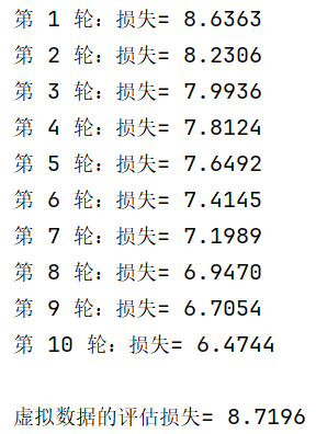
for epoch in range(10):
    optimizer.zero_grad()#清零优化器的梯度
    output = transformer(src_data, tgt_data[:, :-1])#前向传播，得到模型的输出
    loss = criterion(output.contiguous().view(-1, tgt_vocab_size), tgt_data[:, 1:].contiguous().view(-1))
    loss.backward()#反向传播，计算梯度
    optimizer.step()#更新模型参数
    print(f"第 {epoch+1} 轮：损失= {loss.item():.4f}")

# 虚拟数据
src_data = torch.randint(1, src_vocab_size, (5, max_len))  # (batch_size, seq_length)
tgt_data = torch.randint(1, tgt_vocab_size, (5, max_len))  # (batch_size, seq_length)

# 评估循环
transformer.eval()

with torch.no_grad():
    output = transformer(src_data, tgt_data[:, :-1])
    loss = criterion(output.contiguous().view(-1, tgt_vocab_size), tgt_data[:, 1:].contiguous().view(-1))
    print(f"\n虚拟数据的评估损失= {loss.item():.4f}")

难点细讲

1. criterion = nn.CrossEntropyLoss(ignore_index=0):

   • 使用交叉熵损失，并忽略索引为0的标签。这通常用于处理填充位置，假设填充位置的索引为0。

2. optimizer = optim.Adam(transformer.parameters(), lr=0.0001, betas=(0.9, 0.98), eps=1e-9):

   • 使用Adam优化器。lr 是学习率，betas 是Adam优化器的参数，eps 是数值稳定性参数。

3. transformer.train():

   • 将模型设置为训练模式。这会影响某些层的行为，如Dropout和BatchNorm。

4. optimizer.zero_grad():

   • 清零优化器的梯度。在每次迭代开始时，需要清零梯度，以避免梯度累积。

5. output = transformer(src_data, tgt_data[:, :-1]):

   • tgt_data[:, :-1] 表示解码器的输入，去掉最后一个时间步，因为解码器的输入是目标序列的前一个时间步。

6. loss = criterion(output.contiguous().view(-1, tgt_vocab_size), tgt_data[:, 1:].contiguous().view(-1)):

   这个有点难，我们详细讲：

   1. output.contiguous().view(-1, tgt_vocab_size)：
      • output：这是模型的输出张量，形状通常是 (batch_size, seq_len, tgt_vocab_size)，其中：
        • batch_size 是批次大小。
        • seq_len 是序列长度。
        • tgt_vocab_size 是目标词汇表的大小（即目标序列中可能的词汇数量）。
      • contiguous()：这个方法确保张量在内存中是连续存储的。某些操作（如 transpose）可能会使张量变得不连续，而 view 操作要求张量必须是连续的。
      • view(-1, tgt_vocab_size)：这个方法用于改变张量的形状。-1 是一个特殊值，表示自动计算该维度的大小，以确保数据的总元素数量不变。这里，它将 output 张量展平为二维张量，形状为 (batch_size * seq_len, tgt_vocab_size)。
   2. tgt_data[:, 1:].contiguous().view(-1)：
      • tgt_data：这是目标数据张量，形状通常是 (batch_size, seq_len)。
      • tgt_data[:, 1:]：这表示目标序列从第二个时间步开始。这是因为在序列到序列（seq2seq）模型中，解码器的输出对应于目标序列的下一个时间步。例如，如果目标序列是 [a, b, c]，那么第一个时间步的输出应该预测 b，第二个时间步的输出应该预测 c，以此类推。
      • contiguous()：同样，确保张量在内存中是连续存储的。
      • view(-1)：将目标数据展平为一维张量，形状为 (batch_size * seq_len)。

   计算损失

   • criterion：这是一个损失函数，用于计算模型输出和目标数据之间的差异。常见的损失函数包括交叉熵损失（CrossEntropyLoss）等。
   • loss = criterion(...)：将展平后的输出和目标数据传入损失函数，计算损失值。🎉

输出：

💐实践项目

下面，我们实现了一个基于Transformer的机器翻译模型👍！！！

1.库的准备

import math
import torch
import numpy as np
import torch.nn as nn
import torch.optim as optim
import torch.utils.data as Data

2.数据准备

这部分我们的主要目的是将一个数据集（sentences）转换成可以用于序列到序列（Seq2Seq）模型训练的输入格式。具体而言，数据集中每个样本包含一个中文句子和对应的英文翻译。我们需要将这些句子转换为索引，并将数据批量分组。

【1】数据结构

             # Encoder_input   Decoder_input      Decoder_output(预测的下一个字符)
sentences = [['我 是 学 生 P', 'S I am a student', 'I am a student E'], 
             ['我 喜 欢 学 习', 'S I like learning P', 'I like learning P E'],
             ['我 是 男 生 P', 'S I am a boy', 'I am a boy E']]  
# P: 占位符号，如果当前句子不足固定长度用P占位（pad补0）

sentences 是一个列表，包含三个句子对：

• Encoder_input：源语言句子（中文，以单词为单位）。
• Decoder_input：目标语言句子的输入，以 S 开始（表示开始符号）。
• Decoder_output：目标语言句子的输出，以 E 结束（表示结束符号）。

【2】词汇表

# 以下的一个batch中是sentences[0,1]。我们预定每组包含2个样本（如果数据总数不是2的倍数，最后一个组可以包含1个样本）。

src_vocab = {'P': 0, '我': 1, '是': 2, '学': 3, '生': 4, '喜': 5, '欢': 6, '习': 7, '男': 8}  # 词源字典,格式“字：索引”
src_idx2word = {src_vocab[key]: key for key in src_vocab}
src_vocab_size = len(src_vocab)  # 字典字的个数

tgt_vocab = {'S': 0, 'E': 1, 'P': 2, 'I': 3, 'am': 4, 'a': 5, 'student': 6, 'like': 7, 'learning': 8, 'boy': 9} # 生成目标中 'S'是0填充的
idx2word = {tgt_vocab[key]: key for key in tgt_vocab} #把目标字典转换成格式“索引：字”的形式
tgt_vocab_size = len(tgt_vocab)  # 目标字典尺寸

src_len = len(sentences[0][0].split(" "))  # Encoder输入的最大长度 5（对应中文句子字数）
tgt_len = len(sentences[0][1].split(" "))  # Decoder输入输出最大长度 5（英文句子单词数）

• src_vocab：源语言词汇表，将中文词汇映射到唯一的索引。
• tgt_vocab：目标语言词汇表，将英文词汇映射到唯一的索引。
• src_idx2word 和 idx2word：将索引映射回词汇的字典，主要用于可视化或调试😎。

【3】数据预处理&张量转换

# 把sentences 转换成字典索引
def make_data(sentences):
    enc_inputs, dec_inputs, dec_outputs = [], [], []
    for i in range(len(sentences)): 
        enc_input = [[src_vocab[n] for n in sentences[i][0].split()]]
        dec_input = [[tgt_vocab[n] for n in sentences[i][1].split()]]
        dec_output = [[tgt_vocab[n] for n in sentences[i][2].split()]]
        
        enc_inputs.extend(enc_input)
        dec_inputs.extend(dec_input)
        dec_outputs.extend(dec_output)
        
    return torch.LongTensor(enc_inputs), torch.LongTensor(dec_inputs), torch.LongTensor(dec_outputs)

数据预处理

make_data 函数将 sentences 转换为索引列表：

• enc_inputs：源语言句子的索引列表。
• dec_inputs：目标语言句子输入的索引列表（以 S 开始）。
• dec_outputs：目标语言句子输出的索引列表（以 E 结束）。

张量转换

通过 torch.LongTensor，将处理后的数据转换为 PyTorch 的张量格式，以便在模型中使用。

【4】输出示例

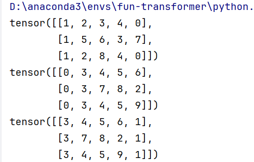
enc_inputs, dec_inputs, dec_outputs = make_data(sentences)  # 这里维度均为3×5，注意长度只是恰巧都为5，enc_inputs、dec_inputs长度可以不一样
print(enc_inputs)
print(dec_inputs)
print(dec_outputs)

输出：

3.数据加载

这里构建一个机器翻译任务的自定义数据集，并定义了一些与Transformer模型相关的配置参数。

# 自定义数据集函数
class MyDataSet(Data.Dataset):
    def __init__(self, enc_inputs, dec_inputs, dec_outputs):#括号内的参数被接收
        super(MyDataSet, self).__init__()
        #保存为类的属性
        self.enc_inputs = enc_inputs
        self.dec_inputs = dec_inputs
        self.dec_outputs = dec_outputs

    def __len__(self):#返回数据集的样本总数
        return self.enc_inputs.shape[0]#enc_inputs 的第0个维度大小

    def __getitem__(self, idx):
        #根据索引 idx，返回对应的 (enc_input, dec_input, dec_output) 三元组
        return self.enc_inputs[idx], self.dec_inputs[idx], self.dec_outputs[idx]
    
loader = Data.DataLoader(MyDataSet(enc_inputs, dec_inputs, dec_outputs), 2, False)
#batch_size=2：每个 batch 的大小为 2。
#shuffle=False：不随机打乱数据。

d_model = 512  # 字 Embedding 的维度
d_ff = 2048  # 前向传播隐藏层维度
d_k = d_v = 64  # K(=Q), V的维度. V的维度可以和K或Q不一样
n_layers = 6  # 有多少个encoder和decoder
n_heads = 8  # Multi-Head Attention设置为8

4.位置编码

【1】 位置嵌入的作用

在序列建模任务中，输入的词的顺序非常重要。然而，Transformer 架构本身并不包含任何关于位置顺序的机制。因此，为了使 Transformer 能够“感知”到词的位置信息😁，我们需要引入一种方法来编码位置信息，这就是位置嵌入的作用。

位置嵌入的核心思想是：

• 为每个位置生成一个唯一💍的向量表示。
• 这些向量与词嵌入向量的维度相同，可以直接相加。

通过这种方式，模型可以同时学习到词的内容信息和它们的位置信息。

【2】位置嵌入的实现细节

位置嵌入的实现基于以下公式：

\[PE_{(pos, 2i)} = \sin\left(\frac{pos}{10000^{2i / d_{\text{model}}}}\right) \]

\[PE_{(pos, 2i+1)} = \cos\left(\frac{pos}{10000^{2i / d_{\text{model}}}}\right) \]

其中：

• pos 是位置（从 0 开始）。
• i 是嵌入维度的索引。
• dmodel 是嵌入的维度（例如 512 或 768）。

具体来说：

• 偶数维度使用正弦函数。
• 奇数维度使用余弦函数。
• 这种设计的好处是：
  • 可以将位置信息编码成连续的向量。
  • 不同的位置向量可以通过加减操作来表示相对位置关系。

【3】初始化函数__init__

• d_model：嵌入的维度（如 512）。
• dropout：用于防止过拟合的 Dropout 概率。
• max_len：支持的最长序列长度（如 5000）。

初始化步骤如下：

1. 生成位置向量表（代码“pos_table”那行）：

   • 对于每个位置 pos，计算其在每个维度 i 的值：
     \[scale=\frac{pos}{10000^{2i / d_{\text{model}}}} \]

• 当 pos == 0 时，所有维度的值均为 0。

2. 应用正弦和余弦函数：

   • 偶数维度（从 0 开始计数）使用正弦函数。
   • 奇数维度使用余弦函数。

3. 转换为 PyTorch 张量：

   • pos_table 是一个形状为 (max_len, d_model) 的张量（5000×512），表示每个位置的嵌入向量。

# 位置嵌入，position Embedding
class PositionalEncoding(nn.Module):
    def __init__(self, d_model, dropout=0.1, max_len=5000):
        super(PositionalEncoding, self).__init__()
        self.dropout = nn.Dropout(p=dropout)
        pos_table = np.array([ [pos / np.power(10000, 2 * i / d_model) for i in range(d_model)] if pos != 0  else np.zeros(d_model)     for pos in range(max_len) ])
        pos_table[1:, 0::2] = np.sin(pos_table[1:, 0::2])  # 正弦函数应用于偶数维度
        pos_table[1:, 1::2] = np.cos(pos_table[1:, 1::2])  # 余弦函数应用于奇数维度
        self.pos_table = torch.FloatTensor(pos_table)  # 转换为 PyTorch 张量
        
        # 输入编码器的只包含语义的enc_inputs: 维度不确定❓
    def forward(self, enc_inputs):
        enc_inputs += self.pos_table[:enc_inputs.size(1),:] #将位置嵌入直接加到词嵌入上
        #enc_inputs.size(1) 的值是 5，表示输入序列的长度（seq_len）
        return self.dropout(enc_inputs)#结果应用 Dropout，防止过拟合

[4]前向传播函数 forward

咳咳，这个为什么加位置嵌入，可以看How Self-Attention with Relative Position Representations works | by ___ | Medium ；有没有别的嵌入，可以看【译】为什么BERT有3个嵌入层，它们都是如何实现的 - d0main - 博客园 😊

5.Mask使用->多头自注意力机制

🍓1. 什么是 Mask（遮蔽）？

在处理文本数据时，句子的长度往往是不一致的。为了方便模型处理，我们会将所有句子填充到相同的长度。通常，我们会用一个特殊的占位符（如 P）来填充不足的部分。

例如，对于输入的句子“我 是 学 生 P”，其中`P`是一个占位符。

然而，这些占位符在实际计算中是没有意义的。为了确保模型在计算时忽略这些占位符，我们需要对它们进行遮蔽（Mask）。遮蔽操作会生成一个布尔矩阵，告诉模型哪些位置是占位符，哪些位置是有意义的。

无论是编码器（Encoder）的输入还是解码器（Decoder）的输入，这些占位符都需要被遮蔽。

🍓2. Mask代码的作用？

这段代码的核心是生成一个遮蔽矩阵🐈（pad_attn_mask），用于告诉模型哪些位置是占位符（P），哪些位置是有意义的词。

这个遮蔽操作的核心代码是seq_k.data.eq(0)。它生成了一个与seq_k大小相同的张量🐈（tensor）。如果seq_k某个位置的值等于0（即占位符），那么对应位置的值就是True，否则就是False。例如，如果输入是seq_data = [1, 2, 3, 4, 0]，那么seq_data.data.eq(0)就会返回[False, False, False, False, True]。

def get_attn_pad_mask(seq_q, seq_k):
    """
    生成遮蔽矩阵，用于忽略占位符（P）。
    
    Args:
        seq_q (_type_): 查询序列，形状为 [batch_size, len_q]。
        seq_k (_type_): 键序列，形状为 [batch_size, len_k]。
        
    Returns:
        _type_: 遮蔽矩阵，形状为 [batch_size, len_q, len_k]，元素为 True 或 False。
    """
    batch_size, len_q = seq_q.size()  # 获取查询序列的批量大小和长度
    # 这些信息用于后续的升维操作，以便生成注意力机制所需的遮蔽矩阵（mask matrix）
    batch_size, len_k = seq_k.size()  # 获取键序列的批量大小和长度
    
    # 生成遮蔽矩阵
    pad_attn_mask = seq_k.data.eq(0)  # 判断 seq_k 中哪些位置是占位符（P=0），返回布尔矩阵 [batch_size, len_k]
    pad_attn_mask = pad_attn_mask.unsqueeze(1)  # 增加一个维度，变为 [batch_size, 1, len_k]
    pad_attn_mask = pad_attn_mask.expand(batch_size, len_q, len_k)  # 扩展为[batch_size, len_q, len_k],这样,每个查询位置（len_q）都可以对应到键序列的每个位置（len_k）😁。
    
    return pad_attn_mask #一个形状为 [batch_size, len_q, len_k] 的布尔矩阵

🎗🎗🎗🎗🎗🎗

• seq_q：查询序列（Query），表示当前需要计算注意力的序列。
• seq_k：键序列（Key），表示需要被查询的序列。
• 在注意力机制中，seq_q 中的每个元素都会与 seq_k 中的每个元素进行交互，计算注意力分数。

根据不同的注意力机制场景，seq_q 和 seq_k 的来源不同：

👒(1) Encoder Self-Attention（编码器自注意力）

• seq_q 和 seq_k：都是编码器的输入（enc_input）。
• 形状：
  • seq_q：[batch_size, enc_len]（enc_len 是中文句子的长度）。
  • seq_k：[batch_size, enc_len]。

👒(2) Decoder Self-Attention（解码器自注意力）

• seq_q 和 seq_k：都是解码器的输入（dec_input）。
• 形状：
  • seq_q：[batch_size, tgt_len]（tgt_len 是英文句子的长度）。
  • seq_k：[batch_size, tgt_len]。

👒(3) Decoder-Encoder Attention（解码器-编码器注意力）

• seq_q：解码器的输入（dec_input）。
• seq_k：编码器的输入（enc_input）。
• 形状：
  • seq_q：[batch_size, tgt_len]（英文句子长度）。
  • seq_k：[batch_size, enc_len]（中文句子长度）。

🎗🎗🎗🎗🎗🎗

🍓3.示例

假设输入的 `seq_k` 是：

seq_k = torch.tensor([[1, 2, 3, 4, 0],  # 第一个句子
                      [1, 5, 6, 3, 7],  # 第二个句子
                      [1, 2, 8, 4, 0]]) # 第三个句子

• seq_k.data.eq(0) 会返回：

  tensor([[False, False, False, False, True],
          [False, False, False, False, False],
          [False, False, False, False, True]])
  

• pad_attn_mask.unsqueeze(1) 会将上述矩阵变为：

  tensor([[[False, False, False, False, True]],
          [[False, False, False, False, False]],
          [[False, False, False, False, True]]])
  

• pad_attn_mask.expand(batch_size, len_q, len_k) 会将上述矩阵扩展为：

  tensor([[[False, False, False, False, True],
           [False, False, False, False, True],
           [False, False, False, False, True],
           [False, False, False, False, True],
           [False, False, False, False, True]],
  
          [[False, False, False, False, False],
           [False, False, False, False, False],
           [False, False, False, False, False],
           [False, False, False, False, False],
           [False, False, False, False, False]],
  
          [[False, False, False, False, True],
           [False, False, False, False, True],
           [False, False, False, False, True],
           [False, False, False, False, True],
           [False, False, False, False, True]]])
  

🍎4.Mask加入Decoder

在中英文翻译过程中，我们首先将整个中文句子“我是学生”输入到编码器（Encoder）中。编码器会逐层处理这个句子，最终输出最后一层的编码结果。

然后，我们开始使用解码器（Decoder）逐步生成英文翻译。在解码器的输入过程中，我们不会一次性将整个英文句子“S I am a student”输入，而是逐步输入。具体步骤如下：

1. 时间步 T0：
   • 输入：“S”（表示开始）。
   • 解码器根据这个输入预测出第一个词“I”。
2. 时间步 T1：
   • 输入：“S”和“I”。
   • 解码器根据这两个词预测出下一个单词“am”。
3. 时间步 T2：
   • 输入：“S”、“I”和“am”。
   • 解码器根据这三个词预测出下一个单词“a”。
4. 依次类推：
   • 直到整个句子“S I am a student E”被逐步生成。

这种逐步输入的方式，使得解码器在生成每个单词时，都能参考之前已经生成的单词，从而更好地理解和生成整个句子😺。

【生成上三角矩阵】

def get_attn_subsequence_mask(seq):
    """
    生成上三角 Attention 矩阵，用于遮蔽未来的信息。

    Args:
        seq (_type_): [batch_size, tgt_len]，目标序列。

    Returns:
        _type_: [batch_size, tgt_len, tgt_len]，上三角矩阵（布尔类型）。
    """
    attn_shape = [seq.size(0), seq.size(1), seq.size(1)]  # 生成上三角矩阵的形状,[batch_size, tgt_len, tgt_len]
    subsequence_mask = np.triu(np.ones(attn_shape), k=1)  # 生成主对角线向上平移一个距离的对角线（下三角包括对角线全为 0）
    subsequence_mask = torch.from_numpy(subsequence_mask).byte()  # 转换为 PyTorch 张量，类型为 byte

    return subsequence_mask

【Scaled Dot-Product Attention】

class ScaledDotProductAttention(nn.Module):
    def __init__(self):
        super(ScaledDotProductAttention, self).__init__()

    def forward(self, Q, K, V, attn_mask):
        """
        计算注意力信息、残差和归一化。

        注意：
            - d_q 和 d_k 一定相同。
            - d_v 和 d_q、d_k 可以不同。
            - len_k 和 len_v 的长度一定相同（翻译任务中，K 和 V 都来自编码器的输出）。

        Args:
            Q (_type_): [batch_size, n_heads, len_q, d_k]，查询矩阵。
            K (_type_): [batch_size, n_heads, len_k, d_k]，键矩阵。
            V (_type_): [batch_size, n_heads, len_v, d_v]，值矩阵。
            attn_mask (_type_): [batch_size, n_heads, len_q, len_k]，注意力遮蔽矩阵（布尔类型）。

        Returns:
            _type_: 
                - context：[batch_size, n_heads, len_q, d_v]，注意力加权后的上下文向量。
                - attn：[batch_size, n_heads, len_q, len_k]，注意力权重矩阵。
        """
        scores = torch.matmul(Q, K.transpose(-1, -2)) / np.sqrt(d_k)  # 计算注意力分数，形状为 [batch_size, n_heads, len_q, len_k]
        # 🐈乘法计算过程~[batch_size, n_heads, len_q, len_k] * [batch_size, n_heads, len_v, d_v] = [batch_size, n_heads, len_q, d_v]
        
        # 将遮蔽矩阵中的 True 位置设置为 -1e9（负无穷），以便在 softmax 中忽略这些位置
        scores.masked_fill_(attn_mask, -1e9)
        
        attn = nn.Softmax(dim=-1)(scores)  # 对最后一个维度进行 softmax，计算注意力权重
        
        context = torch.matmul(attn, V)  # 计算上下文向量，形状为 [batch_size, n_heads, len_q, d_v]

        return context, attn

【多头自注意力机制】

多头自注意力机制（Multi-Head Self-Attention）是 Transformer 模型中的核心组件之一。它的作用是让模型能够同时关注输入序列中的多个位置，从而捕获更丰富的上下文信息。

# 拼接之后 输入fc层 加入残差 Norm
class MultiHeadAttention(nn.Module):
    def __init__(self):
        super(MultiHeadAttention, self).__init__()
        # 定义线性层，用于生成查询（Q）、键（K）和值（V）向量
        self.W_Q = nn.Linear(d_model, d_k * n_heads, bias=False)  # 查询向量
        self.W_K = nn.Linear(d_model, d_k * n_heads, bias=False)  # 键向量
        self.W_V = nn.Linear(d_model, d_v * n_heads, bias=False)  # 值向量

        # 定义线性层，用于将多头注意力的输出拼接后转换回原始维度
        self.fc = nn.Linear(n_heads * d_v, d_model, bias=False)  # 拼接后的全连接层

    def forward(self, input_Q, input_K, input_V, attn_mask):
        """
        多头自注意力机制的前向传播。

        Args:
            input_Q (_type_): 查询矩阵，形状为 [batch_size, len_q, d_model]。
            input_K (_type_): 键矩阵，形状为 [batch_size, len_k, d_model]。
            input_V (_type_): 值矩阵，形状为 [batch_size, len_v, d_model]。
            attn_mask (_type_): 注意力遮蔽矩阵，形状为 [batch_size, len_q, len_k]。

        Returns:
            _type_: 
                - output：注意力机制的输出，形状为 [batch_size, len_q, d_model]。
                - attn：注意力权重矩阵，形状为 [batch_size, n_heads, len_q, len_k]。
        """
        residual, batch_size = input_Q, input_Q.size(0)  # 保存残差连接的输入

        # 1. 生成查询（Q）、键（K）和值（V）向量
        Q = self.W_Q(input_Q).view(batch_size, -1, n_heads, d_k).transpose(1, 2)  # Q: [batch_size, n_heads, len_q, d_k]
        K = self.W_K(input_K).view(batch_size, -1, n_heads, d_k).transpose(1, 2)  # K: [batch_size, n_heads, len_k, d_k]
        V = self.W_V(input_V).view(batch_size, -1, n_heads, d_v).transpose(1, 2)  # V: [batch_size, n_heads, len_v, d_v]

        # 2. 扩展注意力遮蔽矩阵
        attn_mask = attn_mask.unsqueeze(1).repeat(1, n_heads, 1, 1)  # attn_mask: [batch_size, n_heads, len_q, len_k]

        # 3. 计算注意力
        context, attn = ScaledDotProductAttention()(Q, K, V, attn_mask)  # context: [batch_size, n_heads, len_q, d_v]
        # attn: [batch_size, n_heads, len_q, len_k]

        # 4. 拼接多头的结果
        context = context.transpose(1, 2).reshape(batch_size, -1, n_heads * d_v)  # context: [batch_size, len_q, n_heads * d_v]

        # 5. 通过全连接层
        output = self.fc(context)  # d_v fc之后变成 d_model -> [batch_size, len_q, d_model]

        # 6. 残差连接和归一化
        output = nn.LayerNorm(d_model)(output + residual)  # 残差连接 + 归一化

        return output, attn

下面表格是一个补充介绍：

场景	input_Q	input_K	input_V	attn_mask
Encoder Self-Attention	[batch_size, src_len, d_model]	[batch_size, src_len, d_model]	[batch_size, src_len, d_model]	[batch_size, src_len, src_len]
Decoder Self-Attention	[batch_size, tgt_len, d_model]	[batch_size, tgt_len, d_model]	[batch_size, tgt_len, d_model]	[batch_size, tgt_len, tgt_len]
Decoder-Encoder Attention	[batch_size, tgt_len, d_model]	[batch_size, src_len, d_model]	[batch_size, src_len, d_model]	[batch_size, tgt_len, src_len]

里面的input_Q,input_K,input_V是词嵌入、位置嵌入之后的矩阵；attn_mask是注意力遮蔽矩阵——元素全为T or F, T的位置是要掩码(PAD填充)的位置~

6.前馈神经网络

前馈神经网络的主要作用是对输入数据进行非线性变换，以提取更高级的特征。简单来说，它就像一个“加工厂”，把输入的数据“加工”成更有用的特征。😊

工作原理

1. 输入层：

• 输入数据 inputs，通常是一个三维张量，形状为 (batch_size, sequence_length, hidden_size)。
  • batch_size：批量大小，表示一次处理的样本数量。
  • sequence_length：序列长度，表示每个样本的长度。
  • hidden_size：隐藏层的维度，表示每个时间步的特征维度。

2. 第一个全连接层：

   • 输入inputs通过第一个全连接层（通常是一个线性层Linear），得到中间结果hidden。
   • 这个过程可以表示为：\(\text{hidden} = \text{ReLU}(\text{Linear}_1(\text{inputs}))\)
   • 这里使用了 ReLU 激活函数，以引入非线性。ReLU 函数的作用是将负值变为 0，正值保持不变，帮助模型学习更复杂的特征。

3. 第二个全连接层：

   • 中间结果hidden通过第二个全连接层，得到最终输出output。
   • 这个过程可以表示为：\(\text{output} = \text{Linear}_2(\text{hidden})\)
   • 第二个全连接层将中间结果转换回原始维度 d_model，以便与输入数据的维度一致。

4. 残差连接：

   • 将原始输入inputs与前馈神经网络的输出output相加，得到残差结果residual。
   • 这个过程可以表示为：\(\text{residual} = \text{inputs} + \text{output}\)
   • 残差连接的作用是帮助缓解深层网络中的梯度消失问题，使网络更容易训练。它就像一个“捷径”，让梯度可以直接从输出层传递到输入层。😊

5. LayerNorm归一化：

   • 对残差结果residual进行LayerNorm归一化，得到最终输出normalized_output。LayerNorm归一化的作用是对每一句话（即每个序列）进行归一化，而不是对整个批次进行归一化。

   • 这个过程可以表示为:

     \[\text{normalized_output} = \text{LayerNorm}(\text{residual}) \]

代码实现

class FF(nn.Module):
    def __init__(self):
        super(FF, self).__init__()
        self.fc = nn.Sequential(
            nn.Linear(d_model, d_ff, bias=False),  # 第一个全连接层
            nn.ReLU(),  # ReLU 激活函数
            nn.Linear(d_ff, d_model, bias=False)  # 第二个全连接层
        )

    def forward(self, inputs):  # inputs: [batch_size, seq_len, d_model]
        residual = inputs  # 保存残差连接的输入
        output = self.fc(inputs)  # 前馈神经网络的输出
        return nn.LayerNorm(d_model)(output + residual)  # 残差连接 + LayerNorm 归一化
        # [batch_size, seq_len, d_model]

7.编码器和解码器

🌷1. 模型的整体结构

1.1 编码器 (Encoder)

编码器负责将输入的中文句子转换为高维特征表示。它由以下部分构成：

1. 词嵌入层 (Embedding Layer)：
   • 将输入的中文句子索引转换为词向量。
   • 形状：[batch_size, src_len] → [batch_size, src_len, d_model]
2. 位置嵌入层 (Positional Encoding Layer)：
   • 为词向量添加位置信息。
   • 形状：[batch_size, src_len, d_model] → [batch_size, src_len, d_model]
3. 编码器层 (Encoder Layer)：
   • 包含多头自注意力机制和前馈神经网络。
   • 由多个编码器层堆叠而成（通常是 6 个）。

1.2 解码器 (Decoder)

解码器负责将编码器的输出逐步解码为英文句子。它由以下部分构成：

1. 词嵌入层 (Embedding Layer)：
   • 将输入的英文句子索引转换为词向量。
   • 形状：[batch_size, tgt_len] → [batch_size, tgt_len, d_model]
2. 位置嵌入层 (Positional Encoding Layer)：
   • 为词向量添加位置信息。
   • 形状：[batch_size, tgt_len, d_model] → [batch_size, tgt_len, d_model]
3. 解码器层 (Decoder Layer)：
   • 包含两个多头注意力机制（自注意力机制和编码器-解码器注意力机制）和前馈神经网络。
   • 由多个解码器层堆叠而成（通常是 6 个）。

🌺解码器层是解码器的核心组件，包含以下部分：

1. 自注意力机制 (Self-Attention)：
   • 计算解码器输入序列中每个词与其他词的关系。
   • 输入：[batch_size, tgt_len, d_model]
   • 输出：[batch_size, tgt_len, d_model]
2. 编码器-解码器注意力机制 (Encoder-Decoder Attention)：
   • 计算解码器输入序列与编码器输出序列之间的关系。
   • 输入：[batch_size, tgt_len, d_model] 和 [batch_size, src_len, d_model]
   • 输出：[batch_size, tgt_len, d_model]
3. 前馈神经网络 (Feed-Forward Neural Network)：
   • 对每个位置的特征进行非线性变换。
   • 输入：[batch_size, tgt_len, d_model]
   • 输出：[batch_size, tgt_len, d_model]

咳咳咳 ~下面进入代码正题篇😀

🌷2.Encoder Layer (编码器层)

## encoder layer(block)
class EncoderLayer(nn.Module):
    def __init__(self):
        super(EncoderLayer, self).__init__()
        self.enc_self_attn = MultiHeadAttention()  # 多头注意力机制
        self.pos_ffn = FF()  # 前馈神经网络

    def forward(self, enc_inputs, enc_self_attn_mask):  
        '''
        :param enc_inputs: [batch_size, src_len, d_model]，词嵌入和位置嵌入后的输入矩阵
        :param enc_self_attn_mask: [batch_size, src_len, src_len]，元素为 True 或 False，True 表示要掩码（PAD 填充）的位置
        :return:
            enc_outputs: [batch_size, src_len, d_model]，编码器层的输出
            attn: [batch_size, n_heads, src_len, src_len]，注意力权重矩阵
        '''
        # 1. 多头自注意力机制
        enc_outputs, attn = self.enc_self_attn(enc_inputs, enc_inputs, enc_inputs,enc_self_attn_mask)
        # enc_outputs: [batch_size, src_len, d_model],
        # attn: [batch_size, n_heads, src_len, src_len]
        
        # 2. 前馈神经网络
        # 多头自注意力机制（Add & Norm之后）之后，进行FF(Add & Norm)
        enc_outputs = self.pos_ffn(enc_outputs)  
        # enc_outputs: [batch_size, src_len, d_model]
        
        return enc_outputs, attn

🌷3.Encoder (编码器)

class Encoder(nn.Module):
    def __init__(self):
        super(Encoder, self).__init__()
        self.src_emb = nn.Embedding(src_vocab_size, d_model)# 词嵌入层
        self.pos_emb = PositionalEncoding(d_model)# 位置嵌入层
        self.layers = nn.ModuleList(
            [EncoderLayer() for _ in range(n_layers)]
        )# 6 个编码器层

    def forward(self, enc_inputs):
        '''
        :param enc_inputs: [batch_size, src_len]，输入的中文句子索引
        :return:
            enc_outputs: [batch_size, src_len, d_model]，编码器的输出
            enc_self_attns: [batch_size, n_heads, src_len, src_len]，每层的注意力权重
        '''
        # 1. 词嵌入 + 位置嵌入
        enc_outputs = self.src_emb(enc_inputs) 
        #[batch_size, src_len, d_model] 词嵌入(转换成512维度的字向量)
        enc_outputs = self.pos_emb(enc_outputs.transpose(0, 1)).transpose(0, 1)  
        # [batch_size, src_len, d_model] 位置嵌入(字向量上面加上位置信息)
        
        # 2. 生成 PAD 掩码矩阵
        enc_self_attn_mask = get_attn_pad_mask(enc_inputs, enc_inputs)  
        # [batch_size, src_len, src_len]，PAD 掩码(Mask掉句子中的占位符号)
        
        # 3. 通过 6 层编码器(上一层的输出作为下一层的输入)
        enc_self_attns = []# 保存每层的注意力权重
        
        for layer in self.layers:
            enc_outputs, enc_self_attn = layer(enc_outputs, enc_self_attn_mask)  # 每层编码器的输出和注意力权重
            
            enc_self_attns.append(enc_self_attn)  # 保存注意力权重
        
        return enc_outputs, enc_self_attns

# 测试
'''
enc_inputs:
tensor([[1, 2, 3, 4, 0],
        [1, 5, 6, 3, 7],
        [1, 2, 8, 4, 0]])
'''
# enc_outputs, enc_self_attns = Encoder()(enc_inputs)
# print(enc_outputs.shape)    # torch.Size([3, 5, 512])

🌷4.Decoder Layer(解码器层)

# decoder两次调用MultiHeadAttention
class DecoderLayer(nn.Module):
    def __init__(self):
        super(DecoderLayer, self).__init__()
        self.dec_self_attn = MultiHeadAttention()# 自注意力机制
        self.dec_enc_attn = MultiHeadAttention()# 编码器-解码器注意力机制
        self.pos_ffn = FF()# 前馈神经网络

    def forward(self, dec_inputs, enc_outputs, dec_self_attn_mask, dec_enc_attn_mask):
        '''
        :param dec_inputs: [batch_size, tgt_len, d_model]，解码器输入
        :param enc_outputs: [batch_size, src_len, d_model]，编码器输出
        :param dec_self_attn_mask: [batch_size, tgt_len, tgt_len]，解码器自注意力掩码
        :param dec_enc_attn_mask: [batch_size, tgt_len, src_len]，编码器-解码器注意力掩码
        :return:
            dec_outputs: [batch_size, tgt_len, d_model]，解码器输出
            dec_self_attn: [batch_size, n_heads, tgt_len, tgt_len]，自注意力权重
            dec_enc_attn: [batch_size, n_heads, tgt_len, src_len]，编码器-解码器注意力权重
        '''
        # 1. 解码器自注意力机制(传入的 Q，K，V 的值是相同的，都等于dec_inputs)
        dec_outputs, dec_self_attn = self.dec_self_attn(dec_inputs, dec_inputs, dec_inputs,dec_self_attn_mask)
        # dec_outputs: [batch_size, tgt_len, d_model]
        # dec_self_attn: [batch_size, n_heads, tgt_len, tgt_len]

        
        # 2. 编码器-解码器注意力机制(decoder自注意力之后的值作为Q值;K,V来自Encoder的输出)
        dec_outputs, dec_enc_attn = self.dec_enc_attn(dec_outputs, enc_outputs, enc_outputs,dec_enc_attn_mask)
        # dec_outputs: [batch_size, tgt_len, d_model]
        # dec_enc_attn: [batch_size, h_heads, tgt_len, src_len]

        # 3. 前馈神经网络
        dec_outputs = self.pos_ffn(dec_outputs)  # dec_outputs: [batch_size, tgt_len, d_model]
        
        return dec_outputs, dec_self_attn, dec_enc_attn

🌷5.Decoder(解码器)

class Decoder(nn.Module):
    def __init__(self):
        super(Decoder, self).__init__()
        self.tgt_emb = nn.Embedding(tgt_vocab_size, d_model)# 词嵌入层
        self.pos_emb = PositionalEncoding(d_model)# 位置嵌入层
        self.layers = nn.ModuleList([DecoderLayer() for _ in range(n_layers)])# 6 个解码器层

    def forward(self, dec_inputs, enc_inputs, enc_outputs):
        '''
        :param dec_inputs: [batch_size, tgt_len]，输入的英文句子索引
        :param enc_inputs: [batch_size, src_len]，输入的中文句子索引
        :param enc_outputs: [batch_size, src_len, d_model]，编码器的输出
        :return:
            dec_outputs: [batch_size, tgt_len, d_model]，解码器的输出
            dec_self_attns: [batch_size, n_heads, tgt_len, tgt_len]，每层的自注意力权重
            dec_enc_attns: [batch_size, n_heads, tgt_len, src_len]，每层的编码器-解码器注意力权重
        '''
        # 1. 词嵌入 + 位置嵌入
        dec_outputs = self.tgt_emb(dec_inputs)  
        # [batch_size, tgt_len, d_model] 词嵌入
        dec_outputs = self.pos_emb(dec_outputs.transpose(0, 1)).transpose(0, 1)  
        # [batch_size, tgt_len, d_model] 位置嵌入
        
        # 2. 生成 PAD 掩码矩阵
        # PAD：0填充会被Mask掉 
        #（这个例子中decoder是没有加pad的，实际应用中都是有pad填充的）
        # Decoder输入序列的pad mask矩阵：
        #Decoder中0填充的位置是'S'，也就是第一个位置要Mask掉，为true
        dec_self_attn_pad_mask = get_attn_pad_mask(dec_inputs, dec_inputs)
        # [batch_size, tgt_len, tgt_len]，PAD 掩码 T or F 
        
        '''
        此时的一个batch:['S I am a student', 'S I like learning P']
        dec_self_attn_pad_mask： 
        tensor([[[ True, False, False, False, False],
                 [ True, False, False, False, False],
                 [ True, False, False, False, False],
                 [ True, False, False, False, False],
                 [ True, False, False, False, False]],

                [[ True, False, False, False, False],
                 [ True, False, False, False, False],
                 [ True, False, False, False, False],
                 [ True, False, False, False, False],
                 [ True, False, False, False, False]]])'''
        
        # 3. 生成序列掩码矩阵
        # 意义：Masked Self_Attention——当前时刻是看不到未来的信息的
        dec_self_attn_subsequence_mask = get_attn_subsequence_mask(dec_inputs)  
        # [batch_size, tgt_len, tgt_len] ，序列掩码 下三角包括对角线为0，上三角为1
        
        '''
        tensor([[[0, 1, 1, 1, 1],
                 [0, 0, 1, 1, 1],
                 [0, 0, 0, 1, 1],
                 [0, 0, 0, 0, 1],
                 [0, 0, 0, 0, 0]],

                 [0, 1, 1, 1, 1],
                 [0, 0, 1, 1, 1],
                 [0, 0, 0, 1, 1],
                 [0, 0, 0, 0, 1],
                 [0, 0, 0, 0, 0]]], dtype=torch.uint8)'''
        
        # 4. 合并掩码矩阵
        # 操作：Decoder中把两种mask矩阵相加（既屏蔽了pad的信息，也屏蔽了未来时刻的信息🌟）
        # 技术亮点：torch.gt() 比较Tensor1和Tensor2(零矩阵)的每一个元素,并返回一个0-1值.若Tensor1中的元素大于Tensor2中的元素,则结果取1,否则取0
        dec_self_attn_mask = torch.gt((dec_self_attn_pad_mask + dec_self_attn_subsequence_mask),0)  
        # [batch_size, tgt_len, tgt_len]，最终掩码
        
        '''tensor([[[ True,  True,  True,  True,  True],
                    [ True, False,  True,  True,  True],
                    [ True, False, False,  True,  True],    
                    [ True, False, False, False,  True],
                    [ True, False, False, False, False]],

                    [ True,  True,  True,  True,  True],
                    [ True, False,  True,  True,  True],
                    [ True, False, False,  True,  True],
                    [ True, False, False, False,  True],
                    [ True, False, False, False, False]]])'''
        #每行只有False部分dec可见
        # 意义：后面PAD的位置也会注意到前面PAD的位置，当然不包括开始字符'S'。
        
        # 5. 生成编码器-解码器掩码矩阵
        # get_attn_pad_mask主要是🌶enc_inputs的pad mask矩阵(因为enc是处理K,V的，求Attention时是用v1,v2,..vm去加权的，只有把pad对应的v_i的相关系数设为0，这样注意力才不会关注pad向量)，dec_inputs只是提供expand的size的                      
        dec_enc_attn_mask = get_attn_pad_mask(dec_inputs, enc_inputs)  
        # [batc_size, tgt_len, src_len]，编码器-解码器掩码
        
        '''
        此时的一个batch: 'S I am a student' 'S I like learning P'
        下面的tensor是上面两个dec_input样本对应的enc_input的掩码矩阵
        tensor([[[False, False, False, False, False],
                 [False, False, False, False, False],
                 [False, False, False, False, False],
                 [False, False, False, False, False],
                 [False, False, False, False, False]]

                [[False, False, False, False,  True],
                 [False, False, False, False,  True],
                 [False, False, False, False,  True],
                 [False, False, False, False,  True],
                 [False, False, False, False,  True]]
               ])'''
        #每行只有false可见，所以……enc这边是把P消啦？

        # 6. 通过 6 层解码器（上一层的输出作为下一层的输入）
        dec_self_attns, dec_enc_attns = [], []# 保存每层的注意力权重
        for layer in self.layers:
            # dec_outputs: [batch_size, tgt_len, d_model],
            # dec_self_attn: [batch_size, n_heads, tgt_len, tgt_len],
            # dec_enc_attn: [batch_size, h_heads, tgt_len, src_len]
            dec_outputs, dec_self_attn, dec_enc_attn = layer(dec_outputs, enc_outputs, dec_self_attn_mask, dec_enc_attn_mask)
            
            dec_self_attns.append(dec_self_attn)# 保存自注意力权重
            
            dec_enc_attns.append(dec_enc_attn)# 保存编码器-解码器注意力权重
            
        return dec_outputs, dec_self_attns, dec_enc_attns

8.Transformer模型

Transformer 模型的整体结构如下：输入数据先通过编码器（Encoder），再通过解码器（Decoder），最后将解码器的输出进行多分类，分类数为英文字典的长度。具体来说，模型会预测每个位置的单词的概率。

class Transformer(nn.Module):
    def __init__(self):
        super(Transformer, self).__init__()
        self.Encoder = Encoder() # 编码器，负责将输入的中文句子转换为高维特征表示
        self.Decoder = Decoder() # 解码器，负责将编码器的输出逐步解码为英文句子
        self.projection = nn.Linear(d_model, tgt_vocab_size, bias=False) # 投影层，将解码器的输出映射到词汇表大小，用于最终的分类

    def forward(self, enc_inputs, dec_inputs):#前向传播函数
        '''
        :param enc_inputs: [batch_size, src_len]，输入的中文句子索引
        :param dec_inputs: [batch_size, tgt_len]，输入的英文句子索引
        :return:
            dec_logits: [batch_size * tgt_len, tgt_vocab_size]，解码器的输出 logits
            enc_self_attns: [n_layers, batch_size, n_heads, src_len, src_len]，编码器每层的自注意力权重
            dec_self_attns: [n_layers, batch_size, n_heads, tgt_len, tgt_len]，解码器每层的自注意力权重
            dec_enc_attns: [n_layers, batch_size, n_heads, tgt_len, src_len]，解码器每层的编码器-解码器注意力权重
        '''
        # 1. 编码器部分
        enc_outputs, enc_self_attns = self.Encoder(enc_inputs)
        # enc_outputs: [batch_size, src_len, d_model],
        # enc_self_attns: [n_layers, batch_size, n_heads, src_len, src_len]，每层的自注意力权重 

        # 2. 解码器部分
        dec_outputs, dec_self_attns, dec_enc_attns = self.Decoder(dec_inputs, enc_inputs, enc_outputs)
        # dec_outpus    : [batch_size, tgt_len, d_model],每层的注意力权重:
        # dec_self_attns: [n_layers, batch_size, n_heads, tgt_len, tgt_len],
        # dec_enc_attn  : [n_layers, batch_size, tgt_len, src_len]

        # 3. 投影层
        dec_logits = self.projection(dec_outputs)  
        # dec_logits: [batch_size, tgt_len, tgt_vocab_size]
        dec_logits = dec_logits.view(-1, dec_logits.size(-1))  
        # dec_logits: [batch_size*tgt_len, tgt_vocab_size]，以便进行分类
        
        return dec_logits, enc_self_attns, dec_self_attns, dec_enc_attns

9.训练和测试

🐮1.定义模型、损失函数和优化器

# 定义模型、损失函数和优化器
model = Transformer()  # 初始化 Transformer 模型
criterion = nn.CrossEntropyLoss(ignore_index=0)  # 定义损失函数，忽略索引为 0 的位置（PAD）
optimizer = optim.SGD(model.parameters(), lr=1e-3, momentum=0.99)  # 定义优化器，使用 SGD 优化算法

🐮2.训练模型

# 训练模型
for epoch in range(50):  # 训练 50 个 epoch
    for enc_inputs, dec_inputs, dec_outputs in loader:  # 从数据加载器中获取数据(三矩阵维度均为2×5)
        # 前向传播
        outputs, enc_self_attns, dec_self_attns, dec_enc_attns = model(enc_inputs, dec_inputs)
        
        # 计算损失
        # outputs: [batch_size*tgt_len, tgt_vocab_size]
        loss = criterion(outputs, dec_outputs.view(-1))  # 将解码器的输出展平，计算交叉熵损失
        # 打印损失
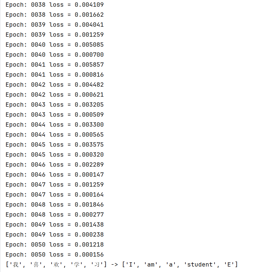
        print('Epoch:', '%04d' % (epoch + 1), 'loss =', '{:.6f}'.format(loss))
        
        # 反向传播和优化
        optimizer.zero_grad()  # 清空梯度
        loss.backward()  # 反向传播
        optimizer.step()  # 更新参数

🐮3.测试模型

# 测试模型
def test(model, enc_input, start_symbol):
    '''
    :param model: 训练好的模型
    :param enc_input: 输入的中文句子索引，形状为 [1, src_len](只取一个例子)
    :param start_symbol: 开始符号的索引
    :return: 预测的英文句子索引
    '''
    # 1. 编码器部分
    enc_outputs, enc_self_attns = model.Encoder(enc_input)  # [1, src_len, d_model] []
    
    # 2. 初始化解码器输入
    dec_input = torch.zeros(1, tgt_len).type_as(enc_input.data)  # [1, tgt_len]
    next_symbol = start_symbol  # 开始符号
    
    # 3. 逐步解码
    for i in range(tgt_len):  # 遍历目标句子的长度
        dec_input[0][i] = next_symbol  # 将当前预测的单词加入解码器输入
        
        # 解码器部分
        dec_outputs, _, _ = model.Decoder(dec_input, enc_input, enc_outputs)  # [1, tgt_len, d_model]
        
        # 投影层
        projected = model.projection(dec_outputs)  # [1, tgt_len, tgt_vocab_size]
        prob = projected.squeeze(0).max(dim=-1, keepdim=False)[1]  # [tgt_len][预测的单词索引]
        
        # 获取下一个单词的索引
        next_word = prob.data[i]  # 获取当前位置的预测单词
        next_symbol = next_word.item()  # 更新下一个单词的索引
    
    return dec_input

这里的投影层维度变换不太好理解，我来疏通一下❤

1. dec_outputs 的形状

• dec_outputs 是解码器的输出，形状为 [batch_size, tgt_len, d_model]。
• 在测试函数中，batch_size 为 1，因此 dec_outputs 的形状为 [1, tgt_len, d_model]。

2. model.projection(dec_outputs)

• model.projection 是一个线性层（nn.Linear），将解码器的输出从 d_model 维度映射到 tgt_vocab_size 维度。
• 输入形状：[1, tgt_len, d_model]
• 输出形状：[1, tgt_len, tgt_vocab_size]

3. projected.squeeze(0)

• squeeze(0) 操作会移除张量的第一个维度（batch_size），因为 batch_size 为 1。
• 输入形状：[1, tgt_len, tgt_vocab_size]
• 输出形状：[tgt_len, tgt_vocab_size]

4. max(dim=-1, keepdim=False)

• max(dim=-1, keepdim=False) 操作会在最后一个维度（tgt_vocab_size）上取最大值。
• 输入形状：[tgt_len, tgt_vocab_size]
• 输出形状：[tgt_len, 2]，其中第一列是最大值(每个位置上的最大概率值)，第二列是最大值的索引(每个位置上预测的单词索引)。

5. [1]

• [1] 表示取最大值的索引。
• 输入形状：[tgt_len, 2]
• 输出形状：[tgt_len]，表示每个位置上预测的单词索引。

🐮4.测试示例

enc_inputs, _, _ = next(iter(loader))# 从数据加载器中获取一个批次的数据，我们这里enc_input只取一个例子,形状为[1, src_len]

# 调用测试函数
# 预测dec_input，dec_input全部预测出来之后，再输入Model预测 dec_output
predict_dec_input = test(model, enc_inputs[1].view(1, -1), start_symbol=tgt_vocab["S"])  
# [1, tgt_len]

# 将预测结果输入模型，得到最终的预测
predict, _, _, _ = model(enc_inputs[1].view(1, -1), predict_dec_input)  
# [tgt_len, tgt_voc_size]

# 获取预测的单词索引
predict = predict.data.max(1, keepdim=True)[1]

# 打印预测结果
print([src_idx2word[int(i)] for i in enc_inputs[1]], '->', [idx2word[n.item()] for n in predict.squeeze()])

预测结果的维度让我看得乱乱的，为大家疏通下：

“predict, _, _, _ = model(enc_inputs[1].view(1, -1), predict_dec_input)”

• enc_inputs[1]：
  • enc_inputs 是一个张量，形状为 [batch_size, src_len]。
  • enc_inputs[1] 表示取第 2 个样本（索引从 0 开始）。
  • 假设 enc_inputs 的形状是 [3, 5]，那么 enc_inputs[1] 的形状是 [5]。
• enc_inputs[1].view(1, -1)：
  • view(1, -1) 💚将 enc_inputs[1] 的形状从 [5] 变为 [1, 5]。
  • 这是为了满足模型输入的形状要求，即 [batch_size, src_len]。
• predict_dec_input：
  • predict_dec_input 是解码器的输入，形状为 [1, tgt_len]。
  • 这是之前通过逐步解码得到的预测结果。
• model(enc_inputs[1].view(1, -1), predict_dec_input)：
  • 将编码器输入和解码器输入传递给模型，得到最终的预测结果。
  • predict 的形状为 [tgt_len, tgt_vocab_size]，表示每个位置上预测的单词的概率分布。

“predict = predict.data.max(1, keepdim=True)[1]”

• predict.data：
  • predict 是一个张量，形状为 [tgt_len, tgt_vocab_size]。
  • predict.data 获取张量的数据部分。
• max(1, keepdim=True)：
  • max(1, keepdim=True) 在第 1 个维度（索引从 0 开始）上取最大值。
  • keepdim=True 💚时，操作后张量的维度会保持不变；当 keepdim=False 时，操作后张量的维度会减少。
  • 返回两个值：
    • 第一个值是最大值，形状为 [tgt_len, 1]。
    • 第二个值是最大值的索引，形状为 [tgt_len, 1]。
• [1]：
  • [1] 表示取第二个值，即最大值的索引。
  • so, 结果的形状为 [tgt_len, 1]。

“print([src_idx2word[int(i)] for i in enc_inputs[1]], '->', [idx2word[n.item()] for n in predict.squeeze()])”

• [src_idx2word[int(i)] for i in enc_inputs[1]]：
  • enc_inputs[1] 是一个张量，形状为 [5]，表示输入的中文句子的索引。
  • src_idx2word 是一个字典，将索引映射为中文单词。
  • 这部分代码将输入的索引转换为中文单词列表。
• [idx2word[n.item()] for n in predict.squeeze()]：
  • predict 的形状为 [tgt_len, 1]，表示每个位置上预测的单词索引。
  • predict.squeeze() 💚将形状从 [tgt_len, 1] 变为 [tgt_len]。
  • idx2word 是一个字典，将索引映射为英文单词。
  • 这部分代码将预测的索引转换为英文单词列表。

输出：

里面的注意力机制作者分析得很棒👍！因为最近在学习Python，就为大家再作一个里面的Python语法难点分析⚡：

1. 类的继承和方法重写

• nn.Module的继承：代码中定义了多个类，如PositionalEncoding, ScaledDotProductAttention, MultiHeadAttention, FF, EncoderLayer, Encoder, DecoderLayer, Decoder, 和Transformer，这些类都继承自torch.nn.Module。这是PyTorch中定义模型的标准方式，通过继承nn.Module并重写forward方法来定义模型的前向传播逻辑。
• forward方法：每个类的forward方法定义了该模块的前向传播逻辑。例如，在PositionalEncoding类中，forward方法实现了位置嵌入的添加和dropout操作。

2. 张量操作

• 张量的创建和转换：使用torch.LongTensor和torch.FloatTensor来创建张量。例如，enc_inputs, dec_inputs, dec_outputs = make_data(sentences)将输入数据转换为长整型张量。
• 张量的维度操作：使用view, transpose, unsqueeze, expand等方法来改变张量的维度。例如，在MultiHeadAttention类中，Q = self.W_Q(input_Q).view(batch_size, -1, n_heads, d_k).transpose(1, 2)将输入张量input_Q的维度从[batch_size, seq_len, d_model]转换为[batch_size, n_heads, seq_len, d_k]。
• 张量的拼接和切片：使用torch.cat和torch.chunk等方法来拼接和切分张量。例如，在MultiHeadAttention类中，context = context.transpose(1, 2).reshape(batch_size, -1, n_heads * d_v)将多头注意力的结果拼接成一个张量。

3. 自定义数据集和数据加载器

• Data.Dataset的继承：定义了MyDataSet类，继承自torch.utils.data.Dataset，并重写了__init__, __len__, 和__getitem__方法。这使得可以自定义数据集的加载方式。
• Data.DataLoader的使用：使用Data.DataLoader来创建数据加载器，方便批量加载数据。例如，loader = Data.DataLoader(MyDataSet(enc_inputs, dec_inputs, dec_outputs), 2, False)创建了一个批量大小为2的数据加载器。

4. 注意力机制的实现

• 多头注意力机制：在MultiHeadAttention类中，实现了多头注意力机制。通过将输入张量Q, K, V分别与权重矩阵W_Q, W_K, W_V相乘，然后将结果分割成多个头，分别计算注意力分数，最后将多头的结果拼接起来并通过一个全连接层。
• 缩放点积注意力：在ScaledDotProductAttention类中，实现了缩放点积注意力机制。通过计算Q和K的点积，然后除以sqrt(d_k)来缩放注意力分数，最后通过softmax函数得到注意力权重。

5. 掩码操作

• PAD掩码：使用get_attn_pad_mask函数来生成PAD掩码，用于屏蔽输入序列中的PAD符号。例如，enc_self_attn_mask = get_attn_pad_mask(enc_inputs, enc_inputs)生成了Encoder自注意力的PAD掩码。
• 序列掩码：使用get_attn_subsequence_mask函数来生成序列掩码，用于屏蔽未来时刻的信息。例如，dec_self_attn_subsequence_mask = get_attn_subsequence_mask(dec_inputs)生成了Decoder自注意力的序列掩码。

6. 模型训练和测试

• 模型训练：使用torch.optim中的优化器（如SGD）和损失函数（如CrossEntropyLoss）来训练模型。例如，optimizer = optim.SGD(model.parameters(), lr=1e-3, momentum=0.99)定义了一个SGD优化器，criterion = nn.CrossEntropyLoss(ignore_index=0)定义了一个交叉熵损失函数。
• 模型测试：定义了test函数来测试模型的翻译能力。例如，predict_dec_input = test(model, enc_inputs[1].view(1, -1), start_symbol=tgt_vocab["S"])使用模型对一个输入句子进行翻译。

7. 代码结构和模块化

• 模块化设计：代码将不同的功能封装成独立的类和函数，如PositionalEncoding, ScaledDotProductAttention, MultiHeadAttention, FF, EncoderLayer, DecoderLayer等。这种模块化设计使得代码更加清晰和易于维护。
• 函数和类的重用：通过定义通用的函数和类，可以在不同的地方重用代码。例如，get_attn_pad_mask和get_attn_subsequence_mask函数在多个地方被调用。

8. 调试和日志&性能优化

• 打印日志：在训练过程中，使用print函数打印每个epoch的损失值，方便监控模型的训练过程。例如，print('Epoch:', '%04d' % (epoch + 1), 'loss =', '{:.6f}'.format(loss))打印了每个epoch的损失值。
• 使用torch.no_grad：在测试阶段，使用torch.no_grad()上下文管理器来禁用梯度计算，从而提高计算效率。例如，在test函数中，with torch.no_grad():禁用了梯度计算。

最重要的，通过详细的注释和模块化设计，代码的可读性和可维护性得到了很好的保证🌹。

这篇笔记我会持续耕耘，含金量很高，谢谢教程的创作者！谢谢群里的助教与热情的小伙伴们，2025新年快乐！！！