时间embedding

左边的公式和 time_embedding(1) 的区别在于它们表示的维度不同。公式中的左边部分是一个概括性公式，用来说明如何为每个时间步 ( t ) 生成时间嵌入。而具体的 time_embedding(1) 展示的是当 ( t = 1 ) 时，如何生成一个更长维度的时间嵌入向量。

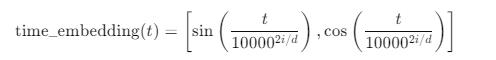
1. 左边公式的含义：

左边的公式表示的是时间步 ( t ) 在不同维度上生成的正弦和余弦值。它用到了参数 ( i ) 和 ( d )，其中：

• ( i ) 是当前的维度索引（不同的 ( i ) 值代表不同的维度），
• ( d ) 是总的嵌入维度。

公式实际上表示，对于嵌入维度的每一个索引 ( i )，我们分别生成正弦和余弦值。这个公式表达了时间步 ( t ) 在不同的维度上如何映射到正弦和余弦值。

2. time_embedding(1) 的具体表示：

time_embedding(1) 展示了当 ( t = 1 ) 时，具体的时间嵌入向量是什么样的。因为时间嵌入是通过正弦和余弦函数生成的，所以它会在嵌入维度的每个索引 ( i ) 上生成两个值：一个是正弦值，另一个是余弦值。

• 对于 ( i = 0 )，我们计算 $ \sin(1) ) 和 ( \cos(1) $，它们是第一个维度的正弦和余弦表示。
• 对于 ( i = 1 )，我们计算 $ \sin\left(\frac{1}{10000^{2 \cdot 1/d}}\right) ) 和 ( \cos\left(\frac{1}{10000^{2 \cdot 1/d}}\right) $，这是第二个维度的正弦和余弦表示。

如此类推，我们继续为后续维度生成对应的正弦和余弦值。每个维度 ( i ) 都会生成一对正弦和余弦值，因此时间嵌入的维度将会是总维度 ( d ) 的两倍。

3. 时间嵌入的维度解释：

具体来说，如果时间嵌入的总维度是 ( d )，那么它将包含 ( d/2 ) 对正弦和余弦值。例如，如果我们生成 6 维的时间嵌入，那么：
\( \text{time_embedding}(1) = \left[ \sin(1), \cos(1), \sin\left(\frac{1}{10000^{2 \cdot 1 / 6}}\right), \cos\left(\frac{1}{10000^{2 \cdot 1 / 6}}\right), \dots \right] \)
总共会包含 6 个元素，即 3 对正弦和余弦值。

总结：

左边的公式是一个概括的生成时间嵌入的方式，而右边展示的是一个具体例子，当时间步 ( t = 1 ) 时，如何生成多对正弦和余弦值。每一对正弦和余弦值都对应着嵌入向量的一个维度，因此最终生成的时间嵌入向量的长度是总维度的两倍。、

累计噪声比例

在扩散模型中，( \alpha_t ) 和 ( \bar{\alpha}_t ) （或者写作 ( \alpha_t^{\text{bar}} )）是两个重要的系数，它们在扩散过程中有不同的定义和作用。

• ( \alpha_t )：是每个时间步 ( t ) 的噪声比例系数。它用于控制当前时间步 ( t ) 上引入噪声的比例。
• ( \bar{\alpha}_t )：是从时间步 0 到时间步 ( t ) 的累计噪声比例。它表示的是到时间步 ( t ) 时为止，嵌入中包含的累计噪声。

1. ( \alpha_t ) 的含义

( \alpha_t ) 表示的是在单个时间步 ( t ) 上引入的噪声比例。每个时间步 ( t ) 都有一个独立的 ( \alpha_t )，用于控制在当前时间步上如何对嵌入进行处理。

在前向扩散过程中，每个时间步 ( t ) 的嵌入更新公式是：
[
h_{t} = \sqrt{\alpha_t} h_{t-1} + \sqrt{1 - \alpha_t} \epsilon
]
其中：

• ( h_{t-1} ) 是上一时间步的嵌入。
• ( \epsilon ) 是从标准正态分布采样的噪声。

通过这个公式，( \alpha_t ) 控制了当前时间步上原始嵌入 ( h_{t-1} ) 和噪声 ( \epsilon ) 之间的权重比例。

2. ( \bar{\alpha}_t ) 的含义

$\bar{\alpha}_t $ 是时间步 ( t ) 之前的累计噪声系数，它表示从第 0 个时间步到第 ( t ) 个时间步的所有噪声的累积效应。具体地，( \bar{\alpha}_t ) 是从时间步 0 到时间步 ( t ) 上每个 ( \alpha_t ) 的乘积：

\( \bar{\alpha}_t = \prod_{i=1}^{t} \alpha_i \)
这意味着，( \bar{\alpha}_t ) 表示嵌入中已经混入的全部噪声的比例。因此，时间步 ( t ) 上的嵌入可以看作是从初始无噪声的嵌入 ( h_0 ) 和噪声 ( \epsilon ) 的组合：

\( h_t = \sqrt{\bar{\alpha}_t} h_0 + \sqrt{1 - \bar{\alpha}_t} \epsilon \)
这表示的是从 ( t = 0 ) 到 ( t ) 时间步的整个噪声添加过程的累积效果。

3. 两者的区别

• ( \alpha_t )：控制每个时间步 ( t ) 单独的噪声比例，即在时间步 ( t ) 中，嵌入和噪声的混合程度。
• ( \bar{\alpha}_t )：是累计噪声比例，它控制了从时间步 0 到 ( t ) 的所有噪声的累积效应，反映了整个扩散过程的总体噪声水平。

4. 举例说明

假设我们有 3 个时间步 ( t = 1, 2, 3 )，每个时间步的 ( \alpha_t ) 分别为：

• $ \alpha_1 = 0.9 $
• $ \alpha_2 = 0.8 $
• $ \alpha_3 = 0.7 $

计算 ( \alpha_t )

这些值表示每个时间步上加入的噪声比例。例如：

• 在时间步 ( t = 1 ) 时，嵌入的更新为：
  \( h_1 = \sqrt{0.9} h_0 + \sqrt{0.1} \epsilon_1 \)
  这里 ( 0.9 ) 控制了原始嵌入和噪声的权重。

• 在时间步 ( t = 2 ) 时，嵌入的更新为：
  \( h_2 = \sqrt{0.8} h_1 + \sqrt{0.2} \epsilon_2 \)

计算 ( \bar{\alpha}_t )

现在，我们计算累计的噪声比例 ( \bar{\alpha}_t )：

• $ \bar{\alpha}_1 = \alpha_1 = 0.9 $
• $ \bar{\alpha}_2 = \alpha_1 \cdot \alpha_2 = 0.9 \times 0.8 = 0.72 $
• $ \bar{\alpha}_3 = \alpha_1 \cdot \alpha_2 \cdot \alpha_3 = 0.9 \times 0.8 \times 0.7 = 0.504 $

这些累计值表示嵌入中从初始状态 ( h_0 ) 到时间步 ( t ) 累积的噪声比例。例如：

• 在时间步 ( t = 3 ) 时，嵌入的计算可以直接表示为：
  \( h_3 = \sqrt{\bar{\alpha}_3} h_0 + \sqrt{1 - \bar{\alpha}_3} \epsilon_3 \)
  这意味着在 ( t = 3 ) 的嵌入中，已经有 ( 1 - 0.504 = 0.496 ) 的嵌入是噪声的贡献，而 $ 0.504 \(是从原始嵌入\) h_0$ 中保留的信息。

5. 总结

• $ \alpha_t $ 控制在当前时间步加入的噪声比例。
• $ \bar{\alpha}_t $ 是从时间步 0 到当前时间步 $t $ 的累积噪声比例。

前者用于控制每一步的嵌入和噪声的混合程度，后者则表示经过$ t $ 个时间步之后，嵌入中的总噪声比例。

在代码中的实现

在你提供的代码中，生成“负样本嵌入”的过程是通过扩散模型的正向扩散机制隐式完成的。下面我详细解释这一过程以及如何从药物嵌入中生成负样本嵌入，并说明是否最终选取了其中的5个。

负样本嵌入的生成方式解释：

1. 噪声嵌入生成（q_sample 方法）：

   • q_sample() 方法从原始的药物嵌入（x_start）生成带噪声的嵌入，其中的噪声是通过高斯噪声（torch.randn_like(x_start)）来添加的，噪声的程度由时间步 t 决定。
   • 在每一个时间步 t，该方法将原始嵌入的一部分（sqrt_alphas_cumprod_t * x_start）与噪声（sqrt_one_minus_alphas_cumprod_t * noise）组合起来。随着 t 的增大，扩散过程逐渐增加噪声。
   • 这个带噪声的嵌入（x_noisy）是原始药物嵌入的“损坏版本”，可以理解为一种“负样本嵌入”，因为它与干净的原始嵌入越来越不同。

2. 预测与损失计算（p_losses 方法）：

   • 在 p_losses() 方法中，模型接收带噪声的嵌入（x_noisy），并通过 encoder 网络预测添加的噪声。
   • 损失函数是根据实际的噪声和模型预测的噪声计算的，使用的是 L1、L2 或 Huber 损失函数。这一损失用于训练模型，帮助它从噪声嵌入中还原原始的嵌入，即去噪。

3. 负样本嵌入的生成：

   • 在这个扩散过程中，并没有明确生成标记为“负样本”的嵌入，而是通过各个时间步 t 生成的带噪声嵌入，可以理解为越来越接近“负样本”的原始嵌入的变体。
   • 模型在扩散过程中尝试预测噪声（从而恢复原始嵌入）的过程可以理解为对比噪声版本（负样本）和干净版本（正样本）的过程。

4. 最终嵌入的选择（p_sample_loop 方法）：

   • 在 p_sample_loop() 方法中，模型从高噪声状态（时间步 t=timesteps）逐步逆向生成嵌入，直到 t=0。这些嵌入存储在 embs 列表中。
   • 随后代码从特定时间步（例如 timesteps/10、timesteps/8 等）选择一些嵌入，最终返回这些嵌入。
   • 也就是说，选择了5个不同时间步中的噪声嵌入，代表了不同噪声程度的药物嵌入。

因此，在你的任务中，所谓的“负样本嵌入”实际上是通过扩散过程生成的不同时间步的带噪声药物嵌入，而最终从这些时间步中选择了5个嵌入，它们分别代表了逐渐去噪的药物嵌入版本。如果你想进一步提取用于对比学习的负样本，可以将中间步骤中的带噪声嵌入视为负样本。

时间嵌入

是的，代码中确实使用了 时间嵌入（time embedding）。具体来说，时间嵌入是在 SinusoidalPosEmb 类和 Encoder 类中实现和应用的。我们来详细分析一下相关部分：

1. SinusoidalPosEmb 类

这个类负责生成 正弦时间嵌入。它的实现方式与 Transformer 模型中的位置编码类似，使用了正弦和余弦函数。

class SinusoidalPosEmb(nn.Module):
    def __init__(self, dim):
        super().__init__()
        self.dim = dim

    def forward(self, x):
        device = x.device
        half_dim = (self.dim // 2) + 1
        emb = math.log(10000) / (half_dim - 1)
        emb = torch.exp(torch.arange(half_dim, device=device) * -emb)
        emb = x[:, None] * emb[None, :]
        emb = torch.cat((emb.sin(), emb.cos()), dim=-1)
        return emb[:,:self.dim]

• SinusoidalPosEmb 接收一个标量 x（对应时间步 t），然后生成一个维度为 dim 的时间嵌入向量。嵌入的计算使用了正弦和余弦函数，目的是为每个时间步 t 提供一个唯一的嵌入表示。
• 正弦和余弦的结合允许模型对时间步的差异具有敏感性，这种表示在扩散模型或类似的生成模型中很常见。

2. Encoder 类中的时间嵌入

在 Encoder 类中，时间嵌入通过 time_mlp 使用。时间嵌入在经过 SinusoidalPosEmb 后，会进一步通过一层多层感知机（MLP）进行非线性变换。

class Encoder(nn.Module):
    def __init__(self, in_ft, out_ft, y=None) -> None:
        super(Encoder, self).__init__()

        self.l1 = Block(in_ft, out_ft) 
        self.l2 = Block(out_ft, out_ft)
        
        sinu_pos_emb = SinusoidalPosEmb(out_ft)
        self.time_mlp = nn.Sequential(
            sinu_pos_emb,
            nn.Linear(out_ft, out_ft),
            nn.GELU(),
            nn.Linear(out_ft, out_ft)
        )

    def forward(self, h, t, y):
        t = self.time_mlp(t)  # 时间嵌入处理
        if y is not None:
            t += y
         
        h = self.l1(h, t) 
        h = self.l2(h, t) 
        
        return h

• self.time_mlp 由 SinusoidalPosEmb 和两个全连接层组成，嵌入首先通过 SinusoidalPosEmb 进行时间步的嵌入计算，随后通过两个线性层进行非线性变换，以便适应模型的其他部分。
• 这个时间嵌入向量 t 在前向传播时会与条件标签 y 相加，并作为条件信息输入到 Block 模块中。

3. 在 Block 中使用时间嵌入

Block 类的 forward 方法中，通过 time 模块对时间嵌入 t 进行了处理，并将其与输入的嵌入 h 结合：

class Block(nn.Module):
    def __init__(self, in_ft, out_ft) -> None:
        super(Block, self).__init__()

        self.lin = nn.Linear(in_ft, out_ft)
        self.time = nn.Sequential(
            nn.SiLU(),
            nn.Linear(out_ft, out_ft * 2)
        )

    def forward(self, h, t):
        t = self.time(t)
        scale, shift = t.chunk(2, dim=1)  # 分为缩放和偏移量
        h = (scale + 1) * h + shift  # 结合时间嵌入和输入嵌入
        return h

• 时间嵌入 t 被分成了缩放因子 scale 和偏移量 shift，然后与输入嵌入 h 进行线性变换 (scale + 1) * h + shift，这是一种条件归一化的方式，确保每个时间步的信息都影响模型的最终输出。

总结

代码中确实使用了 时间嵌入，通过 SinusoidalPosEmb 类生成时间步的嵌入，并在 Encoder 中通过 MLP 进一步处理，最后在 Block 模块中将其用于调节输入的嵌入 h。这些时间嵌入起到了将时间信息（扩散的时间步）融入模型的作用。

labels也就是drug的embedding。是用来预测噪声

在你提供的代码中，labels 的作用主要是在扩散过程中的条件生成部分，特别是在预测噪声时起到条件输入的作用。我们详细分析一下 labels 的具体作用以及它参与的部分。

labels 在代码中的作用

1. 条件扩散模型中的 labels：
   在这个模型中，labels 作为一种条件信息，与时间步 t 一起输入到 Encoder 中进行处理。它代表了一些额外的上下文信息（在你给的上下文中，input 是药物的嵌入，labels 是基因的嵌入），模型会在生成过程中结合 labels 来决定如何调整噪声的预测。

2. 在 Encoder 中使用 labels：
   在 Encoder 的 forward 方法中，labels 会与时间嵌入 t 相加，从而将条件信息融入到时间嵌入中：

   def forward(self, h, t, y):
       t = self.time_mlp(t)  # 时间嵌入处理
   
       if y is not None:
           t += y  # 将 labels 与时间嵌入结合
         
       h = self.l1(h, t) 
       h = self.l2(h, t) 
        
       return h
   

   • 这里的 y 就是传入的 labels（基因嵌入）。当 labels 存在时，它会被加到经过 time_mlp 处理的时间嵌入 t 上。这样做的目的是将 labels 作为条件输入引入扩散模型的生成过程。
   • 加入 labels 后，模型能够根据基因的嵌入信息生成不同的噪声预测结果，从而使生成过程与条件信息（基因嵌入）相关联。

3. 预测噪声中的 labels：
   在 p_losses() 中，模型通过 encoder 预测噪声。在这个过程中，labels 会影响模型对噪声的预测：

   def p_losses(self, x_start, t, labels, noise=None, loss_type="l1"):
       if noise is None:
           noise = torch.randn_like(x_start)
   
       x_noisy = self.q_sample(x_start=x_start, t=t, noise=noise)
    
       predicted_noise = self.encoder(x_noisy, t, labels)  # labels 用于条件输入
   
       if loss_type == 'l1':
           loss = F.l1_loss(noise, predicted_noise)
       elif loss_type == 'l2':
           loss = F.mse_loss(noise, predicted_noise)
       elif loss_type == "huber":
           loss = F.smooth_l1_loss(noise, predicted_noise)
       else:
           raise NotImplementedError()
       return loss
   

   • encoder 使用了 x_noisy（带噪声的药物嵌入）、时间步 t 和 labels 来预测噪声 predicted_noise。在这个过程中，labels 对噪声预测起到条件引导的作用。具体来说，模型根据药物的嵌入和基因的嵌入共同决定应该如何预测噪声。
   • 通过这个条件生成，模型能够在不同的 labels 下产生与之相关联的噪声预测，进而影响生成的样本。

labels 在生成过程中的条件控制

在整个扩散模型的生成过程中，labels 的主要作用是 条件控制。通过把 labels 与时间嵌入结合，模型可以根据基因嵌入（labels）来调整噪声的生成，这样模型在每次生成时都会结合药物和基因的信息。

具体来说：

• 噪声预测中的条件输入：labels 影响了模型如何在每个时间步生成噪声，使得生成的噪声是与 labels 相关的。
• 生成样本中的条件控制：最终生成的样本（通过 p_sample_loop 生成的嵌入）会受到 labels 的控制，使得生成结果与给定的基因信息相匹配。

因此，labels 作为条件信息，直接参与了 噪声预测 和 生成样本 的过程中，确保模型生成的噪声和样本与基因嵌入（labels）相关。

完整实现代码

这段代码实现了一个基于 PyTorch 的条件扩散模型（Conditional Diffusion Model）。扩散模型是一种生成模型，通过逐步向数据添加噪声（前向过程）并训练模型去逆转这个过程（反向过程），从纯噪声中生成数据。

以下是代码的详细步骤和对应的公式解释：

---

1. 导入必要的库

from __future__ import absolute_import, division, print_function
import torch
import torch.nn as nn
import torch.nn.functional as F
import math

这些导入包括基础的数学和神经网络操作，以及未来兼容性支持。

---

2. 定义 Beta 调度函数

Beta 调度函数用于定义在每个时间步添加的噪声量。

2.1 线性 Beta 调度

def linear_beta_schedule(timesteps):
    beta_start = 0.0001
    beta_end = 0.02
    return torch.linspace(beta_start, beta_end, timesteps)

公式：

[
\beta_t = \beta_{\text{start}} + \left( \beta_{\text{end}} - \beta_{\text{start}} \right) \times \frac{t}{T}
]

其中：

• ( \beta_t ) 是第 ( t ) 个时间步的 Beta 值。
• ( T ) 是总的时间步数。

---

3. 辅助函数

3.1 extract 函数

def extract(a, t, x_shape):
    batch_size = t.shape[0]
    out = a.gather(-1, t.cpu())
    return out.reshape(batch_size, *((1,) * (len(x_shape) - 1))).to(t.device)

作用：

从预先计算的数组 a 中提取与时间步 t 对应的值，并将其形状调整为与输入 x 的形状兼容。

---

4. 定义正弦位置嵌入

4.1 SinusoidalPosEmb 类

class SinusoidalPosEmb(nn.Module):
    def __init__(self, dim):
        super().__init__()
        self.dim = dim

    def forward(self, x):
        device = x.device
        half_dim = (self.dim // 2) + 1
        emb = math.log(10000) / (half_dim - 1)
        emb = torch.exp(torch.arange(half_dim, device=device) * -emb)
        emb = x[:, None] * emb[None, :]
        emb = torch.cat((emb.sin(), emb.cos()), dim=-1)
        return emb[:, :self.dim]

公式：

对于输入标量 ( x )，位置嵌入计算为：

[
\text{PE}(x) = \left[ \sin\left(x \cdot \omega_i\right), \cos\left(x \cdot \omega_i\right) \right]_{i=1}^{\frac{D}{2}}
]

其中：

• ( \omega_i = \exp\left( -\frac{\log(10000)}{(\frac{D}{2}-1)} \cdot (i-1) \right) )

---

5. 定义网络基本模块

5.1 Block 类

class Block(nn.Module):
    def __init__(self, in_ft, out_ft):
        super(Block, self).__init__()
        self.lin = nn.Linear(in_ft, out_ft)
        self.time = nn.Sequential(
            nn.SiLU(),
            nn.Linear(out_ft, out_ft * 2)
        )

    def forward(self, h, t):
        t = self.time(t)
        scale, shift = t.chunk(2, dim=1)
        h = (scale + 1) * h + shift
        return h

作用：

• 对输入 h 进行线性变换。
• 使用时间嵌入 t 对特征进行缩放和平移（类似于条件批归一化）。

---

6. 定义编码器

6.1 Encoder 类

class Encoder(nn.Module):
    def __init__(self, in_ft, out_ft, y=None):
        super(Encoder, self).__init__()
        self.l1 = Block(in_ft, out_ft) 
        self.l2 = Block(out_ft, out_ft)
        
        sinu_pos_emb = SinusoidalPosEmb(out_ft)
        self.time_mlp = nn.Sequential(
            sinu_pos_emb,
            nn.Linear(out_ft, out_ft),
            nn.GELU(),
            nn.Linear(out_ft, out_ft)
        )

    def forward(self, h, t, y):
        t = self.time_mlp(t)
        if y is not None:
            t += y
        h = self.l1(h, t) 
        h = self.l2(h, t) 
        return h

作用：

• 使用 Block 进行两层特征提取，每层都与时间嵌入相关。
• 时间嵌入通过 SinusoidalPosEmb 生成，然后经过全连接层和激活函数。
• 如果有条件信息 y，则将其添加到时间嵌入中。

---

7. 定义条件扩散模型

7.1 Diffusion_Cond 类

class Diffusion_Cond(nn.Module):
    def __init__(self, in_feat, out_feat, y):
        super(Diffusion_Cond, self).__init__()
        self.encoder = Encoder(in_feat, out_feat, y)
        self.timesteps = 200
        self.betas = linear_beta_schedule(timesteps=self.timesteps)
        self.alphas = 1. - self.betas
        alphas_cumprod = torch.cumprod(self.alphas, axis=0)
        alphas_cumprod_prev = F.pad(alphas_cumprod[:-1], (1, 0), value=1.0)
        self.sqrt_recip_alphas = torch.sqrt(1.0 / self.alphas)
        self.sqrt_alphas_cumprod = torch.sqrt(alphas_cumprod)
        self.sqrt_one_minus_alphas_cumprod = torch.sqrt(1. - alphas_cumprod)
        self.posterior_variance = (
            self.betas * (1. - alphas_cumprod_prev) / (1. - alphas_cumprod)
        )

初始化参数：

• ( \beta_t )：噪声调度参数，控制每个时间步添加的噪声量。
• ( \alpha_t = 1 - \beta_t )
• 累积乘积 ( \bar{\alpha}t = \prod^t \alpha_s )
• 预计算一些在前向和反向过程中需要的常数。

---

7.2 前向扩散过程 (q_sample 方法)

def q_sample(self, x_start, t, noise=None):
    if noise is None:
        noise = torch.randn_like(x_start)
    sqrt_alphas_cumprod_t = extract(self.sqrt_alphas_cumprod, t, x_start.shape)
    sqrt_one_minus_alphas_cumprod_t = extract(
        self.sqrt_one_minus_alphas_cumprod, t, x_start.shape
    )
    return sqrt_alphas_cumprod_t * x_start + sqrt_one_minus_alphas_cumprod_t * noise

公式：

[
q(\mathbf{x}_t | \mathbf{x}_0) = \sqrt{\bar{\alpha}_t} \mathbf{x}_0 + \sqrt{1 - \bar{\alpha}_t} \mathbf{\epsilon}
]

其中：

• ( \mathbf{x}_0 ) 是初始数据。
• ( \mathbf{\epsilon} \sim \mathcal{N}(0, \mathbf{I}) ) 是标准高斯噪声。
• ( \bar{\alpha}_t ) 是累积乘积。

---

7.3 计算损失 (p_losses 方法)

def p_losses(self, x_start, t, labels, noise=None, loss_type="l1"):
    if noise is None:
        noise = torch.randn_like(x_start)
    x_noisy = self.q_sample(x_start=x_start, t=t, noise=noise)
    predicted_noise = self.encoder(x_noisy, t, labels)
    if loss_type == 'l1':
        loss = F.l1_loss(noise, predicted_noise)
    elif loss_type == 'l2':
        loss = F.mse_loss(noise, predicted_noise)
    elif loss_type == "huber":
        loss = F.smooth_l1_loss(noise, predicted_noise)
    else:
        raise NotImplementedError()
    return loss

公式：

• 预测噪声 ( \hat{\mathbf{\epsilon}}_\theta(\mathbf{x}_t, t) )

• 损失函数：

  • L1 损失：( L = |\mathbf{\epsilon} - \hat{\mathbf{\epsilon}}_\theta(\mathbf{x}_t, t)|_1 )
  • L2 损失：( L = |\mathbf{\epsilon} - \hat{\mathbf{\epsilon}}_\theta(\mathbf{x}_t, t)|_2^2 )

---

7.4 反向采样步骤 (p_sample 方法)

def p_sample(self, model, x, t, labels, t_index, cfg_scale=0):
    betas_t = extract(self.betas, t, x.shape)
    sqrt_one_minus_alphas_cumprod_t = extract(
        self.sqrt_one_minus_alphas_cumprod, t, x.shape
    )
    sqrt_recip_alphas_t = extract(self.sqrt_recip_alphas, t, x.shape)
    predicted_noise = model(x, t, labels)
    if cfg_scale > 0:
        uncond_predicted_noise = model(x, t, None)
        predicted_noise = torch.lerp(uncond_predicted_noise, predicted_noise, cfg_scale)
    model_mean = sqrt_recip_alphas_t * (
        x - betas_t * predicted_noise / sqrt_one_minus_alphas_cumprod_t
    )
    if t_index == 0:
        return model_mean
    else:
        posterior_variance_t = extract(self.posterior_variance, t, x.shape)
        noise = torch.randn_like(x)
        return model_mean + torch.sqrt(posterior_variance_t) * noise 

公式：

• 计算预测的噪声 ( \hat{\mathbf{\epsilon}}_\theta(\mathbf{x}_t, t) )

• 计算模型的均值：

  [
  \mu_\theta(\mathbf{x}_t, t) = \frac{1}{\sqrt{\alpha_t}} \left( \mathbf{x}_t - \frac{\beta_t}{\sqrt{1 - \bar{\alpha}t}} \hat{\mathbf{\epsilon}}\theta(\mathbf{x}_t, t) \right)
  ]

• 如果 ( t > 0 )，则添加噪声项：

  [
  \mathbf{x}{t-1} = \mu\theta(\mathbf{x}_t, t) + \sigma_t \mathbf{z}
  ]

  其中 ( \mathbf{z} \sim \mathcal{N}(0, \mathbf{I}) )，( \sigma_t^2 = \text{posterior_variance}_t )。

---

7.5 反向采样循环 (p_sample_loop 方法)

def p_sample_loop(self, model, shape, y):
    device = next(model.parameters()).device
    b = shape[0]
    emb = torch.randn(shape, device=device)
    embs = []
    for i in reversed(range(0, self.timesteps)):
        emb = self.p_sample(model, emb, torch.full((b,), i, device=device, dtype=torch.long), y, i)
        embs.append(emb)
    embs = embs[::-1]
    steps = [0, int(self.timesteps/10), int(self.timesteps/8), int(self.timesteps/4), int(self.timesteps/2)]
    out = [embs[step] for step in steps]
    return out

作用：

• 从时间步 ( T ) 开始，逐步反向采样至 ( t=0 )。
• 在每个时间步调用 p_sample 方法。

---

7.6 采样接口 (sample 方法)

@torch.no_grad()
def sample(self, shape, y):
    return self.p_sample_loop(self.encoder, shape, y)

作用：

• 对外提供采样接口，生成给定形状和条件 y 的样本。

---

7.7 前向传播 (forward 方法)

def forward(self, input, labels, device): 
    t = torch.randint(0, self.timesteps, (input.shape[0],), device=device).long()
    return self.p_losses(input, t, labels)

作用：

• 随机选择时间步 t，计算损失，用于训练模型。

---

总结

整个流程如下：

1. 前向过程（添加噪声）：

   • 从初始数据 ( \mathbf{x}_0 ) 开始，逐步添加噪声，得到 ( \mathbf{x}_t )。

   • 公式：

     [
     \mathbf{x}_t = \sqrt{\bar{\alpha}_t} \mathbf{x}_0 + \sqrt{1 - \bar{\alpha}_t} \mathbf{\epsilon}
     ]

2. 训练模型预测噪声：

   • 使用编码器模型 ( \hat{\mathbf{\epsilon}}_\theta(\mathbf{x}_t, t) ) 预测添加的噪声。

   • 计算损失：

     [
     L = \mathbb{E}_{t, \mathbf{x}0, \mathbf{\epsilon}} \left[ \left| \mathbf{\epsilon} - \hat{\mathbf{\epsilon}}\theta(\mathbf{x}_t, t) \right|^2 \right]
     ]

3. 反向过程（去噪）：

   • 从纯噪声 ( \mathbf{x}_T ) 开始，逐步去除噪声，生成样本。

   • 在每个时间步，使用模型预测的噪声计算均值，并采样下一步的样本。

4. 条件信息：

   • 条件信息 ( y ) 被添加到时间嵌入中，指导模型生成满足条件的样本。

---

通过上述步骤，模型可以学习如何从噪声中逐步生成逼真的数据，同时满足给定的条件。

我想知道预测噪声时候的xt是用前向时候记录以来使用。还是逆向过程中不断使用新预测的xt

在扩散模型的逆向过程中，预测噪声时使用的 \(\mathbf{x}_t\) 通常是通过逆向推断一步步生成的。具体来说，模型每一步都会基于当前的 \(\mathbf{x}_t\) 预测噪声 \(\hat{\epsilon}_\theta(\mathbf{x}_t, t)\)，然后根据该预测逐步去噪，从 \(\mathbf{x}_t\) 生成 \(\mathbf{x}_{t-1}\)。接下来，在下一个时间步 \(t-1\) 中，新的 \(\mathbf{x}_{t-1}\) 会作为输入进行下一步的噪声预测。

因此，\(\mathbf{x}_t\) 并不是前向过程中直接记录的值，而是通过逆向扩散步骤根据每一步预测得到的。模型会使用每一步生成的 \(\mathbf{x}_{t-1}\)，不断重复这一过程，直到恢复出 \(\mathbf{x}_0\)。

这个过程被称为逐步去噪（denoising），其中每一步的 \(\mathbf{x}_t\) 都基于模型的预测 \(\hat{\epsilon}_\theta(\mathbf{x}_t, t)\) 更新，反向推断逐步减小噪声，最终接近于原始的嵌入 \(\mathbf{x}_0\)。

所以，答案是：在逆向过程中，\(\mathbf{x}_t\) 是逐步使用新预测的 \(\mathbf{x}_t\)，而不是直接使用前向过程中记录的 \(\mathbf{x}_t\)。