弹性波动力学笔记(十)罗格里德斯公式推导
Note: Derivation of the Rodriguez Formula
In this Note, we will derive a formula for \(\mathbf{R}(\widehat{\mathbf{n}},\theta)\) . Consider the three dimensional rotation of a vector \(\boldsymbol{x}\) into a vector \(\boldsymbol{x^{'}}\), which is described algebraically by the equation,
Since we are rotating the vector \(\boldsymbol{x}\) around an axis that is parallel to the unit vector \(\widehat{\boldsymbol{n}}\) , it is convenient to decompose \(\boldsymbol{x}\) into a component parallel to the unit vector \(\widehat{\boldsymbol{n}}\) and a component perpendicular to \(\boldsymbol{n}\). Such a decomposition has the following form,
Note that \(\boldsymbol{x}_{\perp}\) is vector that lives in the three-dimensional plane perpendicular to \(\widehat{\boldsymbol{n}}\) ,whereas \(\boldsymbol{x}_{\|}\) lives one dimensional line parallel to \(\widehat{\boldsymbol{n}}\) . In the above notation, the unbolded symbol \(x_{\|}\) is the length of the vector \(\boldsymbol{x}_{\|}\).

One can obtain convenient formula for \(\boldsymbol{x}_{\|}\) and \(\boldsymbol{x}_{\perp}\) in terms of \(\boldsymbol{x}\) and \(\widehat{\boldsymbol{n}}\) as follows. First, note that
which is equivalent to the statements that \(\boldsymbol{x}_{\perp}\) is perpendicular to \(\widehat{\mathbf{n}}\) and \(\boldsymbol{x}_{\|}\) is parallel to \(\widehat{\boldsymbol{n}}\) . If we now compute the dot product \(\widehat{\boldsymbol{n}} \cdot \boldsymbol{x}\) using equations (1) and (2), then it follows that
Substituting for \(x_{\|}\) back in equation(2) yields,
From this result, we can derive an equation for \(\boldsymbol{x}_{\perp}\). Using equation (2) and (5) ,
We can rewrite the above equation in a fancier way by using a well know vector identity, which yields
Hence, an equivalent form of equation(7) is
To derive a formula for \(\boldsymbol{x}^{\prime}=\mathbf{R}(\widehat{\boldsymbol{n}},\theta)\boldsymbol{x}\) ,the key observation is the following. By decomposing \(\boldsymbol{x}\) according to equation (1), a rotation about an axis that points in the \(\widehat{\boldsymbol{n}}\) direction only rotates \(\boldsymbol{x}_{\perp}\), while leaving \(\boldsymbol{x}_{\|}\) unchanged. Since \(\boldsymbol{x}_{\perp}\) lives a plane, all we need to perform a two-dimensional rotation of \(\boldsymbol{x}_{\perp}\). The end result is the rotated vector,
where \(\boldsymbol{x}_{\perp}=\mathbf{R}(\widehat{\boldsymbol{n}},\theta)\boldsymbol{x}_{\perp}\),\(\boldsymbol{x}_{\|}=\mathbf{R}(\widehat{\boldsymbol{n}},\theta)\boldsymbol{x}_{\|}=\boldsymbol{x}_{\|}\).
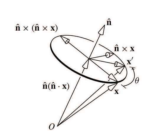
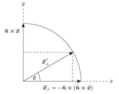
Referring to Figure 1 and 2, we see that the rotated vector \(\boldsymbol{x^{\prime}}_{\perp}\) by an angle \(\theta\) in the two dimensional \(x-y\) plane. In order to check that Figure 2 makes sense as drawn, one should verify that \(\boldsymbol{x}_{\perp}\) is perpendicular to \(\widehat{\boldsymbol{n}}\times{\boldsymbol{x}}\),and both these vectors are mutually perpendicular to the unit vector \(\widehat{\mathbf{n}}\) . Moreover,\(\|\boldsymbol{x}_{\perp}\|=\|\widehat{\boldsymbol{n}}\times\boldsymbol{x}\|\) as indicated in Figure 2.

Figure2
It is convenient to define the following two unit vectors that point along \(x\) and \(y\) axes, respectively,
Note that \(\boldsymbol{\widehat{n}}\cdot\boldsymbol{\widehat{e}}_1=\boldsymbol{\widehat{n}}\cdot\boldsymbol{\widehat{e}}_2=0\), since for any vector \(\boldsymbol{a}\) the cross product \(\boldsymbol{\widehat{n}}\times\boldsymbol{a}\) is perpendicular to \(\boldsymbol{\widehat{n}}\) by the definition of the cross product. Thus, \(\boldsymbol{\widehat{e}}_1\)and\(\boldsymbol{\widehat{e}}_2\) lie in the plane perpendicular to \(\boldsymbol{\widehat{n}}\) as required. To show that \(\boldsymbol{\widehat{e}}_1\)and\(\boldsymbol{\widehat{e}}_2\) are orthogonal, we can use equation(7),
where again we have noted that \(\boldsymbol{\widehat{n}}\times\boldsymbol{x}\) is perpendicular both to \(\boldsymbol{\widehat{n}}\) and to \(\boldsymbol{x}\). Finally, in order to verify that \(\|\boldsymbol{x}_{\perp}\|=\|\boldsymbol{\widehat{n}}\times\boldsymbol{x}\|\), we shall employ the well known vector identity, \(\|a\times b\|=\|a\|^2\|b\|^2-(a\cdot b)^2\). It then follows that
Figure 2 provides a geometric method for finding an expression for \(\boldsymbol{x^{\prime}}_{\perp}\) down to the \(x\) and \(y\) axes in Figure 2,it follows that \(\boldsymbol{x^{\prime}}_{\perp}\) is the vector sum of the two projected vectors. That is,
It is straightforward to verify that \(\|\boldsymbol{x}^{\prime}_{\perp}\|=\|\boldsymbol{x}_{\perp}\|\), which implies that a counterclockwise rotation of \(\boldsymbol{x}_{\perp}\) by an angle \(\theta\) yields \(\boldsymbol{x^{\prime}}_{\perp}\), as required. In particular, in light of equations (12) and (13) one can compute \(\|\boldsymbol{x}^{\prime}\|^2=\boldsymbol{x}^{\prime}\cdot\boldsymbol{x}^{\prime}\) as follows:
Finally, by using equation (5)
since \(\boldsymbol{x}_{\perp}\) lies along the direction of the axis rotation, \(\boldsymbol{\widehat{n}}\) ,and thus does not rotate. Adding the results of equation (14) and (16), we conclude that
Equation 17 is equivalent to the equation \(\boldsymbol{x^{\prime}}=\mathbf{R}(\boldsymbol{\widehat{n}},\theta)\boldsymbol{x}\), where the matrix \(\mathbf{R}(\boldsymbol{\widehat{n}},\theta)\) is axes rotation matrix. To verify this assertion is a straightforward but tedious exercise in expanding out the components of the corresponding cross products. However, if you are comfortable in using the Levi-Civita epsilon symbol, then one can directly obtain the Rodriguez formula by writing equation (17) in terms of components. The components of the cross product are given by
Similarly,using equation (8)
Hence, the components of equation (17)
one can immediately read off the expression for \(R_{ij}(\boldsymbol{\widehat{\boldsymbol{n}}},\theta)\),
Equation (21) is represented as matrix form

 在应力计算中大量需要轴旋转公式计算,因此本笔记给出了罗格里德斯轴旋转公式

 浙公网安备 33010602011771号