弹性波动力学笔记(七) 应力张量简介分解

3.5 Principal directions of stress

Since the stress tensor is real and symmetric, the vector \(\mathbf{e}_{i}\) can be rotated so that \(\tau_{ij}=0,if,i\neq j\), only \(\tau_{11}\) , \(\tau_{22}\), and \(\tau_{33}\) may differ from zero. We will use \(\tau_1\), \(\tau_2\) and \(\tau_3\) for the three diagonal elements. Confusion should not arise by use of the same symbol with a different number of subindex because the two sets of quantities will never be used in the same equation. Let \(\mathbf{a}_{1}\), \(\mathbf{a}_2\), and \(\mathbf{a}_3\) to be represented the unit vectors in the rotated system. In this system

\[\mathcal{T}= \tau_1\mathbf{a}_1\mathbf{a}_1^T+\tau_2\mathbf{a}_2\mathbf{a_2}^T+\tau_3\mathbf{a}_3\mathbf{a}_3^{T} \tag{3.5.1} \]

In matrix form \(\mathcal{T}\) is written as

\[\mathcal{T^{'}}=\left(\begin{array} &\tau_{1} &0 &0 \\ 0 &\tau_2 &0 \\ 0 &0 &\tau_3 \end{array}\right) \tag{3.5.2} \]

In the new (rotated) system the stress vectors are perpendicular to the coordinate planes and the shear stress vanish on these planes. The directions \(\mathbf{a}_1\),\(\mathbf{a}_2\), and \(\mathbf{a}_3\) are known as principal directions of stress, and the planes normal to the principal directions of stress are known as principal planes of stress. In the rotated system the stress vector has a simple expression:

\[\left(\begin{array}{l} T_1 \\ T_2 \\ T_3 \end{array}\right)=\left(\begin{array}{ccc} \tau_1 & 0 & 0 \\ 0 & \tau_2 & 0 \\ 0 & 0 & \tau_3 \end{array}\right)\left(\begin{array}{l} n_1 \\ n_2 \\ n_3 \end{array}\right)=\left(\begin{array}{l} n_1 \tau_1 \\ n_2 \tau_2 \\ n_3 \tau_3 \end{array}\right) \tag{3.5.3} \]

3.6 Isotropic and Deviatoric Components of the Stress Tensor

The stress tensor \(\tau_{ij}\) will be written as the sum of two tensors , one isotropic and other which is with zero trace:

\[\tau_{ij}=P\delta_{ij}+(\tau_{ij}-P\delta_{ij})=P\delta_{ij}+\sigma_{ij} \tag{3.6.1} \]

Where P is a scalar and

\[ \sigma_{ij}=\tau_{ij}-P\delta_{ij} \tag{3.6.2} \]

Because \(\tau_{ij}\) and \(\delta_{ij}\) are symmetric, so is \(\sigma_{ij}\). To determine \(P\) set the trace of \(\sigma_{ij}\) equal to zero:

\[0=\sigma_{ii}=\tau_{ii}-P\delta_{ii}=\tau_{ii}-3P \tag{3.6.3} \]

Therefore

\[P=\frac{\tau_{ii}}{3}=\frac{\tau_{11}+\tau_{22}+\tau_{33}}{3}\tag{3.6.4} \]

In matrix form of equation(3.6.1) is written as

\[\left(\begin{array}{lll} \tau_{11} & \tau_{12} & \tau_{13} \\ \tau_{21} & \tau_{22} & \tau_{23} \\ \tau_{31} & \tau_{32} & \tau_{33} \end{array}\right)=\left(\begin{array}{ccc} P & 0 & 0 \\ 0 & P & 0 \\ 0 & 0 & P \end{array}\right)+\left(\begin{array}{ccc} \tau_{11}-P & \tau_{12} & \tau_{13} \\ \tau_{21} & \tau_{22}-P & \tau_{23} \\ \tau_{31} & \tau_{32} & \tau_{33}-P \end{array}\right) \tag{3.6.4} \]

In dyadic form the equivalent relation is

\[\mathcal{T}=P\mathcal{I}+(\mathcal{T}-P\mathcal{I})=P\mathcal{I}+\mathcal{\Sigma} \tag{3.6.5} \]

The tensor \(P\delta_{ij}\) is known as the isotropic or hydrostatic, or spherical part of the stress tensor. In fluid medium, the stress tensor is

\[ \tau_{ij}=-P\tau_{ij} \tag{3.6.6} \]

where \(P\) is the hydrostatic pressure (a positive number,\(P>0\)).

The tensor \(\sigma_{ij}\) is known as the deviatoric part of the stress tensor. To find the principal directions of \(\sigma_{ij}\) use equation (3.6.1), and let \(v_i\) and \(\lambda\) indicate the eigenvector and the eigenvalue, respectively. This gives

\[\tau_{ij}v_j=\lambda v_i=P\delta_{ij}v_j+\sigma_{ij}v_j \tag{3.6.7} \]

which implies that

\[\sigma_{ij}v_j=(\lambda-P)v_i \tag{3.6.8} \]

Therefore, \(\tau_{ij}\) and \(\sigma_{ij}\) have the same principal directions, while the eigenvalues of \(\sigma_{ij}\) are given by \(\lambda-P\). Because in the rotated system

\[P=\frac{\tau_1+\tau_2+\tau_3}{3} \tag{3.6.9} \]

the eigenvalues of \(\sigma_{ij}\)are

\[\begin{equation} \begin{aligned} \lambda_1=\frac{1}{3}(2\tau_1-\tau_2-\tau_3);\\ \lambda_2=\frac{1}{3}(2\tau_2-\tau_1-\tau_3);\\ \lambda_3=\frac{1}{3}(2\tau_3-\tau_1-\tau_2);\\ \end{aligned} \tag{3.6.10} \end{equation} \]

3.7 Normal and Shearing Stress Vector

Here we will decompose the stress vector \(\mathbf{T}(\mathbf{n})\) into two parts, one, \(\mathbf{T}^{\mathbf{N}}\) , in the direction of \(\mathbf{n}\) and the other, \(\mathbf{T}^{\mathbf{S}}\), perpendicular to \(\mathbf{n}\) (Fig 3.5). \(\mathbf{T}^{\mathbf{N}}\) is known as the shearing stress. The three vectors are on the same plane. From Fig 3.7-1, we see that

\[|\mathbf{T}^{\mathbf{N}}|=\left||\mathbf{T}|\cos{\alpha}\right|=|\mathbf{T}\cdot\mathbf{n}| \tag{3.7.1} \]

Therefore,

\[\mathbf{T}^{\mathbf{N}}=(\mathbf{T}\cdot\mathbf{n})\mathbf{n} \tag{3.7.2} \]

On the other hand,

\[\mathbf{T}=\mathbf{T}^{\mathbf{N}}+\mathbf{T}^{\mathbf{S}} \tag{3.7.3} \]

so that

\[ \mathbf{T}^{\mathbf{S}}=\mathbf{T}-\mathbf{T}^{\mathbf{N}} \tag{3.7.4} \]

and

\[|\mathbf{T}^{\mathbf{S}}|=||\mathbf{T}|\sin{\alpha}|=|\mathbf{n}\times\mathbf{T}|\tag{3.7.5} \]

Equation (3.7.5) does not mean that \(\mathbf{T}^{\mathbf{S}}\) is equal to \(\mathbf{n}\times{\mathbf{T}}\) because the latter is perpendicular to both \(\mathbf{n}\) and the direction of \(\mathbf{T}^{\mathbf{S}}\). However, \(\mathbf{n}\times{\mathbf{T}\times{\mathbf{n}}}\) is in the direction of \(\mathbf{T}^{\mathbf{S}}\) and also has the right absolute value (given in (3.7.5)), so that

\[\mathbf{T}^{\mathbf{S}}_k=\mathbf{n}\times{\mathbf{T}}\times{\mathbf{n}} \tag{3.7.6} \]

To verify that this expression is correct first rewrite equation(3.7.4) in indicial form using equation (3.7.4) in indicial form using equation(3.7.2)

\[\mathbf{T}_{k}^{\mathbf{S}}=\mathbf{T}_{k}-\mathbf{T}_{s}=n_l\tau_{lk}-n_kn_l\tau_{li}n_i=n_l(\tau_{lk}-n_kn_i\tau_{li})\tag{3.7.7} \]

where equation (3.4.11) is used. Next write (3.7.6) in indicial form,

\[\begin{equation} \begin{aligned} (\mathbf{n} \times \mathbf{T} \times \mathbf{n})_k & =\epsilon_{k i j}(\mathbf{n} \times \mathbf{T})_i \mathbf{n}_j=\epsilon_{k i j} \epsilon_{i p q} n_p T_q n_j=-\epsilon_{i k j} \epsilon_{i p q} n_p n_j n_l \tau_{l q} \\ & =-\left(\delta_{k p} \delta_{j q}-\delta_{k q} \delta_{j p}\right) n_p n_j n_l \tau_{l q}=n_j n_j n_l \tau_{l k}-n_k n_j n_l \tau_{l j} \\ & =n_l\left(\tau_{l k}-n_k n_i \tau_{l i}\right), \end{aligned} \tag{3.7.8} \end{equation} \]

because \(n_jn_j=|\mathbf{n}|^2=1\). Since the right-hand sides of equation (3.7.7) and (3.7.8) are equal to each other, equation (3.8.6) is indeed correct.

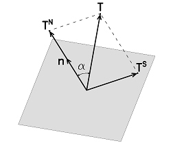
​ Fig. 3.7-1 Decomposition of the stress vector \(\mathbf{T}\) into normal \(\mathbf{T}^{\mathbf{N}}\) and shearing \(\mathbf{T}^{\mathbf{S}}\) components

​