Python共享单车数据分析
一、选题背景:
共享单车在2015年起开始在国内掀起热潮,目前已经逐渐成为了一种新的出行方式,日常生活中短途出行和代步出行,人们更加倾向于选择共享单车,这样既可以免去了等车的时间和花费,也更加的方便快捷、经济实惠,共享单车的出现为我们的生活带来了诸多便利。
二、数据说明:
kaggle的Bike Sharing Demand项目提供了美国某城市的共享单车2011年到2012年的数据集,该数据包括了租车日期,租车季节,租车气温,租车空气湿度等数据。
三、实施过程及代码:
导入库
1 import numpy as np
2 import pandas as pd
3 import calendar
4 import seaborn as sn
5 import matplotlib.pyplot as plt
查看数据大小
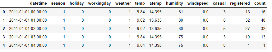
1 #查看数据大小
2 train=pd.read_csv("train.csv")
3 test=pd.read_csv("test.csv")
4 print('训练数据集:',train.shape,'测试数据集:',test.shape)

1 #查看数据情况
2 train.head()
1 #查看数据情况
2 test.head()

比较上述的两个表,我们可以知道test比train少了“casual”,“registered”,“count”三个字段
查看数据总体情况
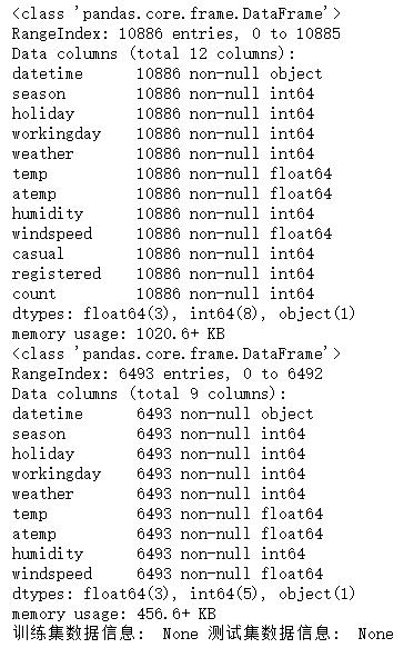
1 #查看数据总体信息
2 print('训练集数据信息: ',train.info(),'测试集数据信息: ',test.info())
数据清洗
时间特征处理
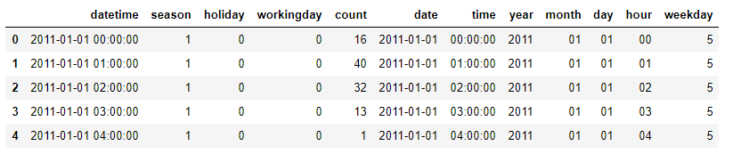
 1 #时间特征处理
 2 #创建一个新的表框
 3 periodDf=train[['datetime','season','holiday','workingday','count']]
 4 #避免报错
 5 periodDf.is_copy = None
 6 #日期处理,把日期提取出来(用匿名函数分离出来)
 7 periodDf['date']=periodDf['datetime'].apply(lambda x: x.split()[0])
 8 periodDf['time']=periodDf['datetime'].apply(lambda x: x.split()[1])
 9 periodDf['year']=periodDf['date'].apply(lambda x: x.split('-')[0])
10 periodDf['month']=periodDf['date'].apply(lambda x: x.split('-')[1])
11 periodDf['day']=periodDf['date'].apply(lambda x: x.split('-')[2])
12 periodDf['hour']=periodDf['time'].apply(lambda x: x.split(':')[0])
13 #星期
14 periodDf['weekday']=periodDf['datetime'].apply(lambda x: pd.to_datetime(x).weekday())
15 #看看处理后的periodDf
16 periodDf.head()
绘图
 1 #绘图
 2 fig1=plt.figure(figsize=(16,4))
 3 ax1=plt.subplot(111)
 4 df1=periodDf.groupby(['month','year']).sum().unstack()['count']#unstack(),将列索引变为行索引
 5 df1.plot(kind='area',ax=ax1,alpha=0.6)
 6 ax1.set_title('2011-2012 bikes sharing demand by month')
 7 ax1.set_xlabel('Figure 1')
 8 ax1.set_xticks(list(range(12)))
 9 ax1.set_xticklabels(['Jan','Feb','Mar','Apr','May','June','July','Aug','Sep','Oct','Nov','DeC'])
10 ax1.set_xlim(0,11)
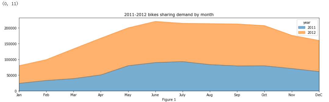
通过上图分析:我们可以看到2012年共享单车的租借数量比2011年是有提升的,一年中6-10月是租借的高峰期。
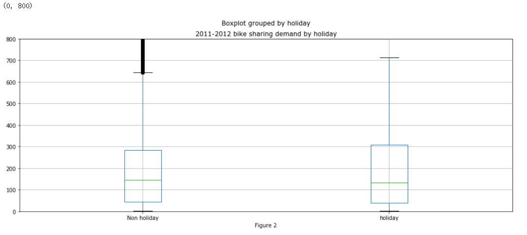
节假日和非节假日租车情况
1 #节假日和非节假日租车情况
2 fig2=plt.figure(figsize=(16,6))
3 ax2=plt.subplot(111)
4 df2=periodDf[['count','holiday']]
5 df2.boxplot(by='holiday',ax=ax2)
6 ax2.set_title('2011-2012 bike sharing demand by holiday')
7 ax2.set_xlabel('Figure 2')
8 ax2.set_xticklabels(['Non holiday','holiday'],rotation='horizontal')
9 ax2.set_ylim(0,800)
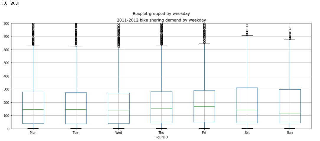
工作日和周末的租车情况
1 #工作日和周末的租车情况
2 fig3=plt.figure(figsize=(16,6))
3 ax3=plt.subplot(111)
4 df3=periodDf[['count','weekday']]
5 df3.boxplot(by='weekday',ax=ax3)
6 ax3.set_title('2011-2012 bike sharing demand by weekday')
7 ax3.set_xlabel('Figure 3')
8 ax3.set_xticklabels(['Mon','Tue','Wed','Thu','Fri','Sat','Sun'], rotation='horizontal')
9 ax3.set_ylim(0,800)
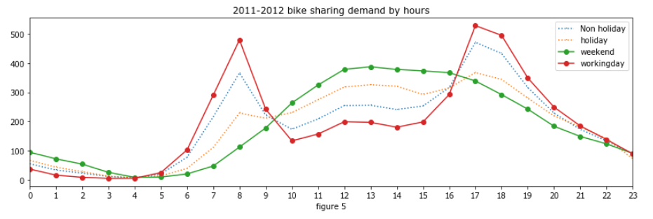
租车数量随季节变化趋势
 1 #租车数量随季节变化趋势
 2 fig5=plt.figure(figsize=(14,4))
 3 ax5=plt.subplot(111)
 4 df51=periodDf.groupby(['hour','holiday']).mean().unstack()['count'].rename(columns={0:'Non holiday',1:'holiday'})
 5 df52=periodDf.groupby(['hour','workingday']).mean().unstack()['count'].rename(columns={0:'weekend',1:'workingday'})
 6 df51.plot(ax=ax5,style=':,')
 7 df52.plot(ax=ax5,style='-o')
 8 ax5.set_title('2011-2012 bike sharing demand by hours')
 9 ax5.set_xlabel('figure 5')
10 ax5.set_xticks(list(range(24)))
11 ax5.set_xticklabels(list(range(24)))
12 ax5.set_xlim(0,23)
13 ax5.legend()
14 plt.show()
非时间特征处理
1 #天气、温度、湿度、风速信息统计
2 climateDf=train[['weather','temp','atemp','humidity','windspeed','count']]
3 climateDf=pd.concat([climateDf,periodDf['hour']],axis=1)
 1 #查看天气和风速对租车数量的影响
 2 fig,axes=plt.subplots(1,2,figsize=(20,6))
 3 ax6=plt.subplot(1,2,1)
 4 df11=climateDf.groupby('weather').sum()['count']
 5 df12=climateDf.groupby('weather').mean()['count']
 6 df1=pd.concat([df11,df12],axis=1).reset_index()
 7 df1.columns=['weather','sum','mean']
 8 df1['sum'].plot(kind='bar',width=0.4,ax=ax6,alpha=0.6,label='')
 9 df1['mean'].plot(style='r-',alpha=0.6,ax=ax6,secondary_y=True,label='mean')
10
11 ax6.set_xlabel('weather')
12 ax6.set_xticks(df1.index)
13 ax6.set_xticklabels(['sunny&cloudy','Fog&overcast','light rain&light snow','bad weather'], rotation='horizontal')
14 ax6.set_ylabel('total')
15 ax6.right_ax.set_ylabel('mean')
16 ax6.set_title('2011-2012 bike sharing demand by weather')
17 ax7=plt.subplot(1,2,2)
18
19 df21=climateDf.groupby('windspeed').sum()['count']
20 df22=climateDf.groupby('windspeed').mean()['count']
21 df2=pd.concat([df21,df22],axis=1).reset_index()
22 df2.columns=['windspeed','sum','mean']
23 df2['sum'].plot(kind='area',ax=ax7,alpha=0.7,color='orange',label='')
24 df2['mean'].plot(style='-',alpha=0.6,color='red',ax=ax7,secondary_y=True,label='mean')
25 ax7.set_xlabel('windspeed')
26 ax7.set_ylabel('total')
27 ax7.right_ax.set_ylabel('mean')
28 ax7.set_title('2011-2012 bike sharing demand by windspeed')
29 plt.show()

左图柱状图反应了不同天气下租车总数的变化,大雨大雪大雾这种恶劣天气最低。折现图反应了各种天气下平均租车数量,异常的是平均数量在恶劣天气下反而显著增加;
右图反应了随着风速变大,租车的总数量趋向于0,但平均租车数却最高。
1 train[train['weather']==4]

1 train[train['windspeed']>50]
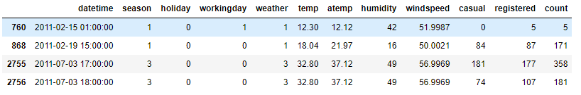
通过查看原始数据发现,这种极端情况的数据仅为个例,所以造成了异常现象
湿度、温度对租车数量的影响
 1 #查看湿度、温度对租车数量的影响
 2 fig=plt.subplots(1,2,figsize=(20,8))
 3
 4 ax1=plt.subplot(1,2,1)
 5 df1=climateDf[['humidity','count']]
 6 ax1.scatter(df1['humidity'],df1['count'],s=df1['count']/5, c=df1['count'],marker='.',alpha=0.6)
 7 ax1.set_title('2011-2012 bike sharing demand by humidity')
 8 ax1.set_xlabel('humidity')
 9 ax1.set_ylabel('count')
10
11 ax2=plt.subplot(1,2,2)
12 df2=climateDf[['temp','count']]
13 ax2.scatter(df2['temp'],df2['count'],s=df1['count']/5, c=df1['count'],marker='.',alpha=0.6)
14 ax2.set_title('2011-2012 bike sharing demand by temperature')
15 ax2.set_xlabel('temperature')
16 ax2.set_ylabel('count')
17 plt.show()
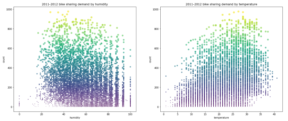
最适合的湿度为30-40附近,温度越高,租车数量减少,最适合的温度在25-30左右
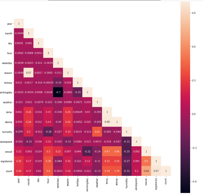
租车数量和其它变量的相关性
1 #查看租车数量和其它变量的相关性
2 df=pd.concat([periodDf.iloc[:,-5:].astype(int),train.iloc[:,1:]],axis=1)
3 corrDf=df.corr()
4 mask=np.array(corrDf)
5 mask[np.tril_indices_from(mask)]=False
6 fig=plt.figure(figsize=(15,15))
7 sn.heatmap(corrDf,mask=mask,annot=True,square=True)
8 plt.show()
完整代码
  1 import numpy as np
  2 import pandas as pd
  3 import calendar
  4 import seaborn as sn
  5 import matplotlib.pyplot as plt
  6
  7 #查看数据大小
  8 train=pd.read_csv("train.csv")
  9 test=pd.read_csv("test.csv")
 10 print('训练数据集:',train.shape,'测试数据集:',test.shape)
 11
 12 #查看数据情况
 13 train.head()
 14 test.head()
 15
 16 #查看数据总体信息
 17 print('训练集数据信息: ',train.info(),'测试集数据信息: ',test.info())
 18
 19
 20 #时间特征处理
 21 #创建一个新的表框
 22 periodDf=train[['datetime','season','holiday','workingday','count']]
 23 #避免报错
 24 periodDf.is_copy = None
 25 #日期处理,把日期提取出来(用匿名函数分离出来)
 26 periodDf['date']=periodDf['datetime'].apply(lambda x: x.split()[0])
 27 periodDf['time']=periodDf['datetime'].apply(lambda x: x.split()[1])
 28 periodDf['year']=periodDf['date'].apply(lambda x: x.split('-')[0])
 29 periodDf['month']=periodDf['date'].apply(lambda x: x.split('-')[1])
 30 periodDf['day']=periodDf['date'].apply(lambda x: x.split('-')[2])
 31 periodDf['hour']=periodDf['time'].apply(lambda x: x.split(':')[0])
 32 #星期
 33 periodDf['weekday']=periodDf['datetime'].apply(lambda x: pd.to_datetime(x).weekday())
 34 #看看处理后的periodDf
 35 periodDf.head()
 36
 37
 38 #绘图
 39 fig1=plt.figure(figsize=(16,4))
 40 ax1=plt.subplot(111)
 41 df1=periodDf.groupby(['month','year']).sum().unstack()['count']#unstack(),将列索引变为行索引
 42 df1.plot(kind='area',ax=ax1,alpha=0.6)
 43 ax1.set_title('2011-2012 bikes sharing demand by month')
 44 ax1.set_xlabel('Figure 1')
 45 ax1.set_xticks(list(range(12)))
 46 ax1.set_xticklabels(['Jan','Feb','Mar','Apr','May','June','July','Aug','Sep','Oct','Nov','DeC'])
 47 ax1.set_xlim(0,11)
 48
 49
 50 #节假日和非节假日租车情况
 51 fig2=plt.figure(figsize=(16,6))
 52 ax2=plt.subplot(111)
 53 df2=periodDf[['count','holiday']]
 54 df2.boxplot(by='holiday',ax=ax2)
 55 ax2.set_title('2011-2012 bike sharing demand by holiday')
 56 ax2.set_xlabel('Figure 2')
 57 ax2.set_xticklabels(['Non holiday','holiday'],rotation='horizontal')
 58 ax2.set_ylim(0,800)
 59
 60
 61 #工作日和周末的租车情况
 62 fig3=plt.figure(figsize=(16,6))
 63 ax3=plt.subplot(111)
 64 df3=periodDf[['count','weekday']]
 65 df3.boxplot(by='weekday',ax=ax3)
 66 ax3.set_title('2011-2012 bike sharing demand by weekday')
 67 ax3.set_xlabel('Figure 3')
 68 ax3.set_xticklabels(['Mon','Tue','Wed','Thu','Fri','Sat','Sun'], rotation='horizontal')
 69 ax3.set_ylim(0,800)
 70 fig4=plt.figure(figsize=(14,4))
 71 ax4=plt.subplot(111)
 72 df4=periodDf.groupby(['hour', 'season']).mean().unstack()['count']
 73 df4.columns=['Spring','Summer','Fall','Winter']
 74 df4.plot(ax=ax4, style='--.')
 75 ax4.set_title('2011-2012 bike sharing demand by hours')
 76 ax4.set_xlabel('Figure 4')
 77 ax4.set_xticks(list(range(24)))
 78 ax4.set_xticklabels(list(range(24)))
 79 ax4.set_xlim(0,23)
 80
 81
 82 #租车数量随季节变化趋势
 83 fig5=plt.figure(figsize=(14,4))
 84 ax5=plt.subplot(111)
 85 df51=periodDf.groupby(['hour','holiday']).mean().unstack()['count'].rename(columns={0:'Non holiday',1:'holiday'})
 86 df52=periodDf.groupby(['hour','workingday']).mean().unstack()['count'].rename(columns={0:'weekend',1:'workingday'})
 87 df51.plot(ax=ax5,style=':,')
 88 df52.plot(ax=ax5,style='-o')
 89 ax5.set_title('2011-2012 bike sharing demand by hours')
 90 ax5.set_xlabel('figure 5')
 91 ax5.set_xticks(list(range(24)))
 92 ax5.set_xticklabels(list(range(24)))
 93 ax5.set_xlim(0,23)
 94 ax5.legend()
 95 plt.show()
 96
 97
 98 #天气、温度、湿度、风速信息统计
 99 climateDf=train[['weather','temp','atemp','humidity','windspeed','count']]
100
101
102 #查看天气和风速对租车数量的影响
103 fig,axes=plt.subplots(1,2,figsize=(20,6))
104 ax6=plt.subplot(1,2,1)
105 df11=climateDf.groupby('weather').sum()['count']
106 df12=climateDf.groupby('weather').mean()['count']
107 df1=pd.concat([df11,df12],axis=1).reset_index()
108 df1.columns=['weather','sum','mean']
109 df1['sum'].plot(kind='bar',width=0.4,ax=ax6,alpha=0.6,label='')
110 df1['mean'].plot(style='r-',alpha=0.6,ax=ax6,secondary_y=True,label='mean')
111 ax6.set_xlabel('weather')
112 ax6.set_xticks(df1.index)
113 ax6.set_xticklabels(['sunny&cloudy','Fog&overcast','light rain&light snow','bad weather'], rotation='horizontal')
114 ax6.set_ylabel('total')
115 ax6.right_ax.set_ylabel('mean')
116 ax6.set_title('2011-2012 bike sharing demand by weather')
117 ax7=plt.subplot(1,2,2)
118 df21=climateDf.groupby('windspeed').sum()['count']
119 df22=climateDf.groupby('windspeed').mean()['count']
120 df2=pd.concat([df21,df22],axis=1).reset_index()
121 df2.columns=['windspeed','sum','mean']
122 df2['sum'].plot(kind='area',ax=ax7,alpha=0.7,color='orange',label='')
123 df2['mean'].plot(style='-',alpha=0.6,color='red',ax=ax7,secondary_y=True,label='mean')
124 ax7.set_xlabel('windspeed')
125 ax7.set_ylabel('total')
126 ax7.right_ax.set_ylabel('mean')
127 ax7.set_title('2011-2012 bike sharing demand by windspeed')
128 plt.show()
129 climateDf=pd.concat([climateDf,periodDf['hour']],axis=1)
130 train[train['weather']==4]
131 train[train['windspeed']>50]
132
133
134 #查看湿度、温度对租车数量的影响
135 fig=plt.subplots(1,2,figsize=(20,8))
136 ax1=plt.subplot(1,2,1)
137 df1=climateDf[['humidity','count']]
138 ax1.scatter(df1['humidity'],df1['count'],s=df1['count']/5, c=df1['count'],marker='.',alpha=0.6)
139 ax1.set_title('2011-2012 bike sharing demand by humidity')
140 ax1.set_xlabel('humidity')
141 ax1.set_ylabel('count')
142 ax2=plt.subplot(1,2,2)
143 df2=climateDf[['temp','count']]
144 ax2.scatter(df2['temp'],df2['count'],s=df1['count']/5, c=df1['count'],marker='.',alpha=0.6)
145 ax2.set_title('2011-2012 bike sharing demand by temperature')
146 ax2.set_xlabel('temperature')
147 ax2.set_ylabel('count')
148 plt.show()
149
150
151 #查看租车数量和其它变量的相关性
152 df=pd.concat([periodDf.iloc[:,-5:].astype(int),train.iloc[:,1:]],axis=1)
153 corrDf=df.corr()
154 mask=np.array(corrDf)
155 mask[np.tril_indices_from(mask)]=False
156 fig=plt.figure(figsize=(15,15))
157 sn.heatmap(corrDf,mask=mask,annot=True,square=True)
158 plt.show()
总结
经过上述的可视化分析,我们对共享单车租车数据有了大致的把握,对数据特征之间的关系有了初步的了解。季节、小时、月份、工作日非工作日、天气状况、温度、湿度、风速等特征对总体需求量有相关性。总的来说,效果还是蛮不错的,后面会再多加强这方面的知识。

 浙公网安备 33010602011771号