Lecture9 Neural Networks Learning

Lecture9 Neural Networks:Learning

Cost function

Neural Network (Classifification)

\(L\) = total no. of layer in network

\(S_l\) = no. of units (not counting bias unit) in layer \(l\)

Binary classification

y = 0 or 1 , 1 output unit

Multi-class classification (K classes)

\(y \in \mathbb{R}^K\) e.g. \(\left[\begin{matrix}1\\0\\0\\0\end{matrix}\right]\),\(\left[\begin{matrix}0\\1\\0\\0\end{matrix}\right]\),\(\left[\begin{matrix}0\\0\\1\\0\end{matrix}\right]\),\(\left[\begin{matrix}0\\0\\0\\1\end{matrix}\right]\),K output units

Cost function

logistic regression

\[J(\Theta) = \frac{1}{m}[\sum^m_{i=1} - y^{(i)}\ log(h_\Theta(x^{(i)})) - (1-y^{(i)}) log(1-h_\Theta(x^{(i)}))]+\frac{\lambda}{2m}\sum_{j=1}^n\theta_j^2 \]

Neural network:

\[h_\Theta(x) \in \mathbb{R}^K\ \ (h_\Theta(x))_i = i^{th} output\\ J(\Theta) = \frac{1}{m}[\sum^m_{i=1}\sum_{k=1}^K - y_k^{(i)}\ log(h_\Theta(x^{(i)}))_k - (1-y_k^{(i)}) log(1-h_\Theta(x^{(i)}))_k]+\frac{\lambda}{2m}\sum_{l=1}^{L-1}\sum_{i=1}^{s_l}\sum_{j=1}^{s_l+1}(\theta^{(l)}_{ji})^2 \]

Backpropagation algorithm

Gradient computation

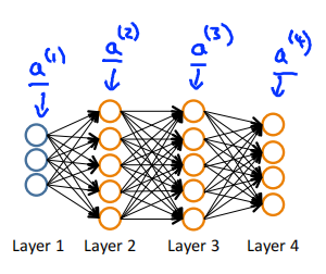
Given one training example(x,y),Forward propagation:

\[\begin{align} a^{(1)} & = x \\ z^{(2)} & = \Theta^{(1)} a^{(1)} \\ a^{(2)} & = g(z^{(2)})\ (add\ a_0^{(2)}) \\ z^{(3)} & = \Theta^{(2)} a^{(2)} \\ a^{(3)} & = g(z^{(3)})\ (add\ a_0^{(3)}) \\ z^{(4)} & = \Theta^{(3)} a^{(3)} \\ a^{(4)} & = h_\Theta(x) = g(z^{(4)}) \\ \end{align} \]

Backpropagation algorithm

Intuition: \(\delta_j^{(l)}\) = "error" of node \(j\) in layer \(l\) ,Formally

\[\delta_j^{(l)} = \frac{\partial}{\partial z_j^{(l)}}J \]

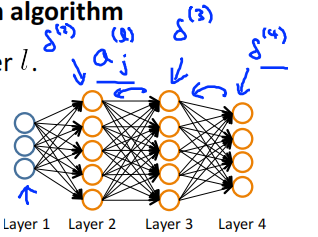
For each output unit (layer L = 4)

\[\begin{align} \delta^{(4)}_j & = a_j^{(4)} - y_j \Rightarrow \delta^{(4)} = a^{(4)}-y\\ \delta^{(3)} & = ((\Theta^{(3)})^T\delta^{(4)}).*g'(z^{(3)})\\ \delta^{(2)} & = ((\Theta^{(2)})^T\delta^{(3)}).*g'(z^{(2)})\\ \\ g'(z^{(3)}) & =a^{(3)}.*(1-a^{(3)})\\ g'(z^{(2)}) & =a^{(2)}.*(1-a^{(2)}) \end{align} \]

Step of Algorithm

set \(\Delta_{ij}^{(l)} = 0\) (for all l,i,j)

For i = 1 to m

​ Set \(a^{(1)} = x^{(i)}\)

​ Perform forward propagation to compute \(a^{(l)}\) for \(l=2,3,\cdots,L\)

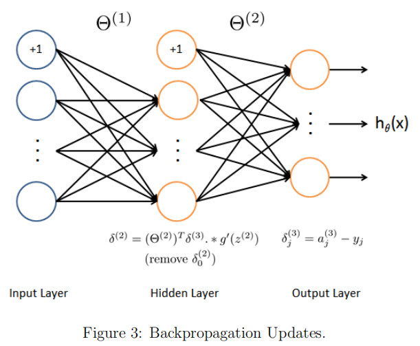
​ Using \(y^{(i)}\),compute \(\delta^{(L)} = a^{(L)}-y^{(i)}\)

​ compute \(\delta^{(L-1)},\delta^{(L-2)},\cdots,\delta^{(2)}\)

​ \(\Delta^{(l)}_{ij} += a^{(l)}_j\delta^{(l+1)}_i\)

\(D_{ij}^{(l)} = \frac{1}{m}\Delta_{ij}^{(l)}+\lambda\Theta_{ij}^{(l)}\ \ if\ j \neq 0\)

\(D_{ij}^{(l)} = \frac{1}{m}\Delta_{ij}^{(l)}\ \ if\ j = 0\)

\(\frac{\partial}{\partial\Theta_{ij}^{(l)}}J(\Theta)=D_{ij}^{(l)}\)

Backpropagation intuition

对\(\delta^{(L)} = a^{(L)}-y\)的推导

损失函数选择 交叉熵函数，激活函数选择sigmoid函数。

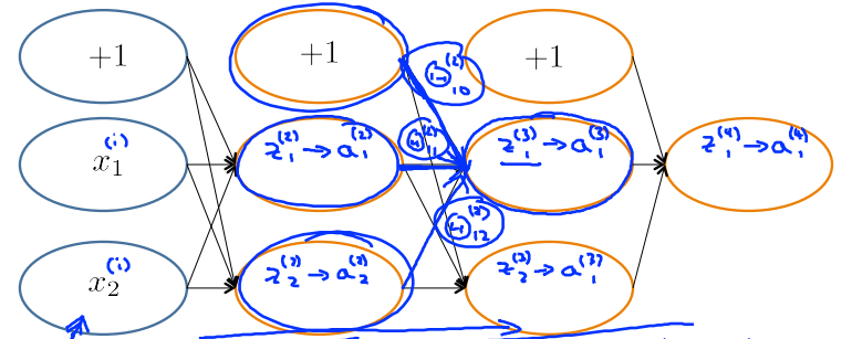
对于如下图所示的神经网络求$$\delta^{(3)}$$

即对下函数求导。此处选用一个样本作为例子，y为该样本的真实值的向量，z3也为向量。

求导过程如下

\[\begin{align} J_\theta(z_3) = &\sum_{k=1}^{K}-y_k\ log(\frac{1}{1+e^{-z_k^{(3)}}}) - (1-y_k) log(1-\frac{1}{1+e^{-z_k^{(3)}}})\\ J'_\theta(z_k^{(3)})= & -y_k\ (1+e^{-z_k^{(3)}})\frac{-1}{(1+e^{-z_k^{(3)}})^2}e^{-z_k^{(3)}}(-1)-(1-y)\frac{1+e^{-z_k^{(3)}}}{e^{-z_k^{(3)}}}(-1)\frac{-1}{(1+e^{-z_k^{(3)}})^2}e^{-z_k^{(3)}}(-1) \\ = & - \frac{y_ke^{-z_k^{(3)}}}{1+e^{-z_k^{(3)}}} - \frac{y_k-1}{1+e^{-z_k^{(3)}}} \\ = & -\frac{(1+e^{-z_k^{(3)}})y_k-1}{1+e^{-z_k^{(3)}}} \\ = & \frac{1}{1+e^{-z_k^{(3)}}} - y_k \\ = & h_k - y_k \\ = & a^{(3)}_k - y_k \end{align} \]

对\(((\Theta^{(l)})^T\delta^{(l+1)})\)的理解

求得\(\delta^{(l+1)}\)之后，要求得\(\delta^{(l)}\)，需要求得\(\frac{\partial}{\partial a^{(l)}}J\)。使用链式法则进行推导

前向传播过程中，\(z_1^{(3)}=\Theta^{(2)}_{10}\times1+\Theta^{(2)}_{11}a^{(2)}_1+\Theta^{(2)}_{12}a^{(2)}_2\)，\(z_2^{(3)}\)同理

所以反向传播时候,\(\frac{\partial}{\partial a_1^{(2)}}J = \Theta_{11}^{(2)} \delta^{(3)}_1 + \Theta_{21}^{(2)} \delta^{(3)}_2\)，\(\frac{\partial}{\partial a_2^{(2)}}J\)同理

所以

\[\frac{\partial}{\partial a^{(l)}}J=((\Theta^{(l)})^T\delta^{(l+1)}) \]

求\(\delta^{(l)}\)时，再次运用链式法则

因为\(a^{(l)}=g(z^{(l)})\)，即\(a_i^{(l)}=\frac{1}{1+e^{(-z^{(l)}_i)}}\)所以

\[\begin{align} \delta^{(l)} &= \frac{\partial}{\partial a^{(l)}}\frac{\partial a^{(l)}}{\partial z^{(l)}}J \\ &= ((\Theta^{(l)})^T\delta^{(l+1)}).*g'(z^{(l)}) \\ &= ((\Theta^{(l)})^T\delta^{(l+1)}).*(a^{(l)}.*(1-a^{(l)})) \end{align} \]

Gradient Checking

gradApprox = (J(theta+EPSILON) - J(theta-EPSILON))/(2*EPSILON)

\(\theta \in \mathbb{R}^n\) (E.g. \(\theta\) is "unrolled" version of \(\theta^{(1)}\), \(\theta^{(2)}\), \(\theta^{(3)}\)）

\[\theta = [\theta_1,\theta_2,\theta_3,\cdots,\theta_n]\\ \frac{\partial}{\partial\theta_1}J(\theta)\approx\frac{J(\theta_1+\epsilon,\theta_2,\theta_3,\cdots,\theta_n)-J(\theta_1-\epsilon,\theta_2,\theta_3,\cdots,\theta_n)}{2\epsilon}\\ \vdots\\ \frac{\partial}{\partial\theta_n}J(\theta)\approx\frac{J(\theta_n,\theta_2,\theta_3,\cdots,\theta_n+\epsilon)-J(\theta_1,\theta_2,\theta_3,\cdots,\theta_n-\epsilon)}{2\epsilon}\\ \]

Random initialization

Zero initialization

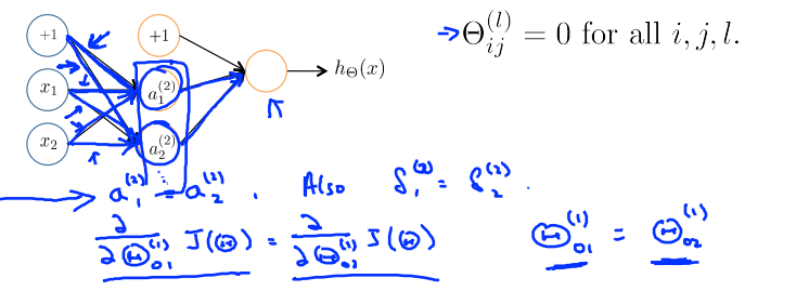
正向传播的时候，\(a_1^{(2)} = a_2^{(2)}\)，所以

\[\delta_1^{(2)}=\delta_2^{(2)}\\ \frac{\partial}{\partial\Theta_{01}^{(1)}}J(\Theta)=\frac{\partial}{\partial\Theta_{01}^{(1)}}J(\Theta)\\ \Theta_{01}^{(1)}=\Theta_{02}^{(1)} \]

After each update,parameters corresponding to inputs going into each of two hidden units are identical

Symmetry breaking

Initialize each \(\Theta_{ij}^{(l)}\) to a random value in \([-\epsilon,\epsilon]\)