Honors Calculus Notes for [5 Integration]

Definition

Def. 5.1 Riemann integral (黎曼积分)

Let \([a, b]\) be a given interval, with \(a<b\). Let \(P\) be a partition (割分) of \([a, b]\):

\[P: a=x_0\leq x_0\leq x_1\leq \cdots\leq x_{n-1}\leq x_n=b \]

Suppose \(f\) is a bounded real-valued function defined on \([a,b]\), so we assume that there exists \(m\) and \(M\) such that \(m\leq f(x)\leq M\) for \(x\in[a, b]\). On each subinterval \([x_{i-1}, x_i]\), put

\[m_i=\inf_{x_{i-1}\leq x\leq x_i}f(x),\text{ }\ M_i=\sup_{x_{i-1}\leq x\leq x_i} f(x) \]

Write \(\Delta x_i:=x_i-x_{i-1}, 1\leq i\leq n\). Form the lower sum (下和) and the upper sum （上和）

\[L(P, f)=\sum_{i=1}^nm_i\Delta x_i,\text{ } U(P, f)=\sum_{i=1}^nM_i\Delta x_i \]

respectively. For each fixed partition \(P\),

\[(b-a)m\leq L(P, f)\leq U(P, f)\leq (b-a)M \]

so that the numbers \(\lbrace L(P, f)\rbrace\) and \(\lbrace U(P, f)\rbrace\) form bounded sets.

Denote the lower integral (下积分) and the upper integral (上积分), respectively:

\[\underline{\int}_{a}^{b} f \text{d} x=\sup_{P}L(P, f), \text{ }\overline{\int}_{a}^{b} f \text{d} x=\inf_{P}L(P, f) \]

When two values are equal, we represent the common value using the notation

\[\int_{a}^{b} f(x)\text{d} x \text { or } \int_{a}^{b} f\text{d} x \]

which is referred to as the Riemann integral or the definite integral (定积分) of \(f\) over the interval \([a, b]\). The function \(f\) is referred to as the integrand (被积函数).

If the integral exists, we say that \(f\) is Riemann integrable (黎曼可积) on \([a, b]\), and write \(f\in \mathscr{R}[a, b]\).

Def. 5.2 Refinement (细化)

The partition \(Q\) is a refinement (细化) of \(P\) if every point of \(P\) is a point of \(Q\), that is, \(Q\supset P\).

Given two partitions, \(P_1\) and \(P_2\), we say that \(P_1\cup P_2\) is their common refinement (共同细化).

Suppose \(Q\) is any refinement of partition \(P\) of \([a,b]\). Then

\[L(P, f)\leq L(Q, f)\leq U(Q, f)\leq U(P, f) \]

Def. 5.3 Riemann Sum (黎曼和)

The Riemann integral was defined originally by Riemann similarly to the concept in Condition 2,
expressed as the limit

\[\lim_{||P||\rightarrow 0}\sum_{i=1}^nf(x_i^*)\Delta x_i=I \]

where \(x_i^*\in[x_{i-1}, x_i]\) is an arbitrary point in the subintervals. Here, the summation \(\sum_{i=1}^nf(x_i^*)\Delta x_i\) is called the Riemann sum (黎曼和), and \(||P||=\max_{1\leq i\leq n}\Delta x_i\) denotes the mesh (细度) of the partition \(P\).

Riemann v.s. Darboux

It can be shown that both Riemann's and Darboux's definitions ultimately describe the same concept of integration for functions that satisfy specific criteria; however, they differ in their methods and applications.

Darboux's definition is considered a more foundational approach that emphasizes bounding functions, whereas Riemann's definition concentrates on evaluating function values at particular points.

Def. 5.4 Uniformly Continuous (一致连续)

For a function \(f:=I\rightarrow \mathbb R\), where \(I\) is a interval and \(I\subset \mathbb R\). If for any \(\epsilon >0\), there exists \(\delta>0\) s.t. for any \(x_1, x_2\in I\), \(|x_1-x_2|<\delta\), \(|f(x_1)-f(x_2)|<\epsilon\), we call \(f\) is uniformly continuous (一致连续) on \(I\).

(comment: consider \(f(x)=\frac{1}{x}, x\in(0, 1)\))

• \(f\) is continuous on a closed interval \(I\) \(\Leftrightarrow\) \(f\) is uniformly continuous a closed interval on \(I\).

Proof

• Part 1 (\(\Leftarrow\))

If the uniformly continuous holds, we have for any \(\epsilon>0\), there exists \(\delta>0\) s.t. for any \(x_1, x_2\in I\), \(|x_1-x_2|<\delta\), \(|f(x_1)-f(x_2)|<\epsilon\).

Then for a fixed \(x_0\), for any \(\epsilon >0\), there exists \(\delta>0\) s.t. for any \(|x-x_0|<\delta, x\in I\), \(|f(x)-f(x_0)|<\epsilon\), which implies that \(f\) is continuous on \(x_0\).

We apply this analysis on every point in \(I\), then we can obtain that \(f\) is continuous on \(I\).

• Part 2 (\(\Rightarrow\))

If the continuous holds, we have for any \(x_0\in I\), \(\forall \epsilon >0\), \(\exists \delta>0\) s.t. \(\forall |x-x_0|<\delta, x\in I, |f(x)-f(x_0)|<\epsilon\).

If there exists \(\epsilon >0\) s.t. \(\forall \delta_n>0\) , \(\exists x_{1, n}, x_{2, n}\in I, |x_{1, n}-x_{2, n}|<\delta_n, |f(x_{1, n})-f(x_{2, n})|\geq \epsilon\)

Assuming that \(\forall n\in \mathbb N, \delta_n>\delta_{n+1}\), then we form two sequence \(\{x_{1, n}\}\) and \(\{x_{2, n}\}\) from above, and assuming that \(x_{1, n}>x_{2, n}\) holds for all \(n\in\mathbb N\).

\(\because \lim_{n\rightarrow \infty}\delta_n=0\),

\(\therefore \lim_{n\rightarrow \infty} (x_{1, n}-x_{2, n})=0\).

According to Bolzano-Weusetrass Theorem, we can select a subsequence \(\{x_{1, n_k}\}\) from \(\{x_{1, n}\}\) that converges. Let \(\lim_{k\rightarrow\infty} x_{1, n_k}=x^*\).

\(\because \lim_{n\rightarrow \infty} (x_{1, n}-x_{2, n})=0\)

\(\therefore \lim_{k\rightarrow \infty} (x_{1, n_k}-x_{2, n_k})=0\) (we consider \(\{x_{1, n}-x_{2, n}\}\) as a sequence that converges).

\(\therefore \{x_{2, n_k}\}\) also converges and \(\lim_{k\rightarrow\infty} x_{2, n_k}=x^*\in I\).

That implies when \(\delta\rightarrow 0\), \(|\lim_{x\rightarrow x^{*+}}f(x)-\lim_{x\rightarrow x^{*-}}f(x)|\geq\epsilon>0\), which means \(\lim_{x\rightarrow x^{*+}} f(x)\neq \lim_{x\rightarrow x^{*-}}f(x)\).

Thus \(f\) is not continuous on \(x^*\), which conflicts with \(f\) is continuous on \(I\).

Thus \(f\) is uniformly continuous on \(I\).

[知乎] 数学分析中的反例（2）——连续和一致连续 - Ra1n F0rest

[知乎] 一致连续性(1):(非)一致连续性的判定 - 铁球

Def. 5.5 Indefinite Integral (不定积分)

Given a function \(f:I\rightarrow \mathbb R\) defined on an open interval \(I\). If \(f\) is an antiderivative of \(f\) on \(I\), then the expression \(F(x)+C\), where \(C\) is an arbitrary constant, is called the indefinite integral (不定积分) of \(f(x)\) with respect to \(x\) and is denoted by

\[\int f\text{d}x=F(x)+C \text{ or } \int f(x)\text{d}x=F(x)+C \]

The function \(f(x)\) is called the integrand (被积函数), \(C\) is the constant of integration (积分常数)

Def. 5.6 Improper Integral (反常积分)

Improper Integral of Type 1 (第一类反常积分)

• Suppose \(f\) is a function defined on an interval \([a, \infty)\) such that \(f\) is integrable over \([a, t]\) for any \(t>a\). The improper integral (反常积分) is defined as a limit of a definite integral as follows:

\[\int_{a}^{\infty}f(x)\text{d}x=\lim_{t\rightarrow\infty}f(x)\int_{a}^{t}\text{d}x \]

• When the limit exists, we say the improper integral is convergent (收敛); otherwise, it is divergent (发散).

• Suppose \(f\) is a function defined on an interval \((-\infty, a]\) such that \(f\) is integrable over \([t, a]\) for any \(t<a\). The improper integral is defined as a limit of a definite integral as follows:

\[\int_{-\infty}^{a}f(x)\text{d}x=\lim_{t\rightarrow -\infty}f(x)\int_{t}^{a}\text{d}x \]

• Suppose \(f\) is a function defined on \((-\infty, \infty)\) such that \(f\) is integrable on any bounded closed interval. We define the improper integral:

\[\int_{-\infty}^{\infty}f(x)\text{d}x=\int_{-\infty}^{a}\text{d}x+\int_{a}^{\infty}\text{d}x \]

• where \(a\) is any fixed real number.

Improper Integral of Type 2 (第二类反常积分)

• Suppose \(f\) is a function defined on an interval \([a, b)\) such that \(f\) is integrable over \([a, t]\) for any \(t\in (a, b)\), and suppose \(f\) is unbounded in \([t, b)\). We define the improper integral as a limit of a definite integral as follows:

\[\int_{a}^{b}f(x)\text{d}x=\lim_{t\rightarrow b^{-}}\int_{a}^{t}f(x)\text{d}x \]

• When the limit exists, we say the improper integral is convergent; otherwise, it is divergent.

• Suppose \(f\) is a function defined on an interval \((b, a]\) such that \(f\) is integrable over \([t, a]\) for any \(t\in (b, a)\), and suppose \(f\) is unbounded in \((b, t]\). We define the improper integral as a limit of a definite integral as follows:

\[\int_{b}^{a}f(x)\text{d}x=\lim_{t\rightarrow b^{+}}\int_{t}^{a}f(x)\text{d}x \]

• Suppose \(f\) is a function defined on an interval \([a, c]\), possibly not at \(b\) where \(b\in(a, c)\). If \(f\) is unbounded near \(b\), and if \(\int_{a}^{b}f(x)\text{d}x\) and \(\int_{b}^{c}f(x)\text{d}x\) are convergent, then we define

\[\int_{a}^{c}f(x)\text{d}x=\int_{a}^{b}f(x)\text{d}x+\int_{b}^{c}f(x)\text{d}x \]

Example

• Show \(\int_{0}^{\infty}e^{-x}\text{d}x\) converges and find its value.

  • \(\int_{0}^{t}e^{-x}\text{d}x=1-e^{-t}\)

  • \(\int_{0}^{\infty}e^{-x}\text{d}x=\lim_{t\rightarrow \infty}\int_{0}^{t}e^{-x}\text{d}x=\lim_{t\rightarrow \infty}(1-e^{-t})=1\)

• Determine whether \(\int_{-\infty}^{0}\cos x\text{d}x\) converges.

  • \(\int_{t}^{0}\cos x\text{d}x=(\sin x)|_{x=t}^{0}=-\sin t\)

  • \(\lim_{n\rightarrow \infty}\sin(-2n\pi)=0\neq 1=\lim_{n\rightarrow \infty}\sin(-2n\pi+\frac{\pi}{2})\)

  • Hence, the given improper integral diverges.

• Determine whether \(\int_{0}^{1}\ln x\text{d}x\) converges, and if it does, find its value.

  • \(\int_{t}^{1}\ln x\text{d}x=(x\ln x)|_{x=t}^{1}-\int_{t}^{1}x\cdot\frac{1}{x}\text{d}x=-t\ln t-(1-t)=-t\ln t-1+t\)

  • \(\int_{0}^{1}\ln x\text{d}x=\lim_{t\rightarrow 0^{+}}\int_{t}^{1}\ln x\text{d}x=\lim_{t\rightarrow 0^{+}}(-t\ln t-1+t)=-1\)

• Consider \(\int_{0}^{1}x^p\text{d}x \text{ } (p<0, p\neq -1)\). Find the values of \(p\) for which the improper integral converges.

  • \(\int_{t}^{1}x^p\text{d}x=\frac{x^{p+1}}{p+1}|_{x=t}^{1}=\frac{1-t^{p+1}}{p+1}\)

  • \(\lim_{t\rightarrow 0^{+}}\frac{1-t^{p+1}}{p+1}=\infty\) for \(p<-1\)

  • \(\lim_{t\rightarrow 0^{+}}\frac{1-t^{p+1}}{p+1}=\frac{1}{p+1}\) for \(-1<p<0\)

Proposition & Theorem

Theo. 5.1 the Integrability criterion (可积性判据)

A function \(f\in\mathscr{R}[a,b]\) if and only if the integrability criterion (可积性判据) holds:

\[\forall \epsilon >0, \exists P \text{ of } [a,b] \text{ such that } U(P,f)-L(P,f)=\sum_{i=1}^n\left(\omega_{[x_{i-1}, x_i]}(f)\right)\Delta x<\epsilon \]

Here \(\omega_{[x_{i-1}, x_i]}(f):=M_i-m_i\) is called the oscillation (振荡) of \(f\) on \([x_{i-1}, x_i]\), with

\[M_i=\sup_{x_{i-1}\leq x\leq x_i}f(x), \text{ }m_i=\inf_{x_{i-1}\leq x\leq x_i}f(x), \]

Proof Theo 5.1

Part 1 (\(\Rightarrow\))

Suppose \(f\in \mathscr{R}[a,b]\). For \(\epsilon>0\), by the definition of the upper and lower integrals, there exists partitions \(P_1\) and \(P_2\) such that

\[\underline\int_{a}^bf\text{d}x-L(P_1,x)<\frac{\epsilon}{2} \]

and

\[-\overline\int_{a}^bf\text{d}x+U(P_2,x)<\frac{\epsilon}{2} \]

Let \(P\) be the common refinement of \(P_1\) and \(P_2\). Since \(\underline\int_{a}^bf\text{d}x=\overline\int_{a}^bf\text{d}x=\int_{a}^bf\text{d}x\), we have

\[U(P, f)\leq U(P_2, f)<\int_{a}^bf\text{d}x+\frac{\epsilon}{2}<L(P_1, f)+\epsilon\leq L(P, f)+\epsilon \]

so that

\[U(P, f)-L(P, f)<\epsilon \]

Part 2 (\(\Leftarrow\))

Suppose the integrability criterion holds. For every \(\epsilon >0\), there exists a partition \(P\) such that \(U(P, f)-L(P, f)<\epsilon\). Since

\[L(P, f)\leq \underline\int_{a}^bf\text{d}x\leq \overline\int_{a}^bf\text{d}x\leq U(P, f) \]

we obtain

\[0\leq \overline\int_{a}^bf\text{d}x-\underline\int_{a}^bf\text{d}x<\epsilon \]

Because \(\epsilon\) is arbitrary, we have

\[\overline\int_{a}^bf\text{d}x-\underline\int_{a}^bf\text{d}x=0 \]

so that \(f\in \mathscr{R}[a,b]\)

Necessary and Sufficient Conditions for Integrability (可积性的充分必要条件)

Condition 1

• \(\forall \epsilon>0, \exists P\text{ of }[a,b]\) such that

\[\sum_{i=1}^{n}|f(s_i)-f(t_i)|\Delta x_i<\epsilon \]

for any \(s_i, t_i\in [x_{i-1}, x_i], i=1, 2,\cdots,n\).

Proof Condition 1

Part 1 (\(\Rightarrow\))

Suppose \(f\in \mathscr{R}[a,b]\). By the integrability criterion, there exists a partition \(P\) of \([a, b]\), such that \(U(P, f)-L(P, f)<\epsilon\). For any \(s_i, t_i\in[x_{i-1}, x_i], i=1, 2, \cdots, n\), since

\[|f(s_i)-f(t_i)|\leq M_i-m_i \]

we have

\[\sum_{i=1}^n|f(s_i)-f(t_i)|\Delta x_i\leq \sum_{i=1}^n(M_i-m_i)\Delta x_i=\sum_{i=1}^n(\omega_{[x_i-1, x_i]}(f))\Delta x_i=U(P, f)-L(P, f)<\epsilon \]

That is, for the same partition \(P\), Condition 1 for integrability holds.

Part 2 (\(\Leftarrow\))

Suppose that Condition 1 for integrability holds. Thus, for every \(\epsilon >0\) there exists a partition \(P:a=x_0\leq x_1\leq \cdots \leq x_n\leq b\), such that

\[\sum_{i=1}^n|f(s_i)-f(t_i)|\Delta x_i<\frac{1}{3}\epsilon \]

for any choice of \(s_i, t_i\in[x_{i-1}, x_i], i=1, 2, \cdots, n\). For each \(i\), choose \(s_i^*, t_i^*\in[x_{i-1}, x_i]\), such that

\[f(s_i^*)>M_i-\frac{\frac{1}{3}\epsilon}{b-a+c} \]

\[f(t_i^*)<m_i+\frac{\frac{1}{3}\epsilon}{b-a+c} \]

\((c \text{ is a constant and } c>0)\)

Thus,

\[\begin{aligned} U(P, f)-L(P, f)&=\sum_{i=1}^n\left(\omega_{[x_{i-1}, x_i]}\right)\\\\ &=\sum_{i=1}^nM_i\Delta x_i-\sum_{i=1}^nm_i\Delta x_i\\\\ &\leq \sum_{i=1}^n\left[f(s_i^*)+\frac{\frac{1}{3}\epsilon}{b-a+c}\right]\Delta x_i+\sum_{i=1}^n\left[\frac{\frac{1}{3}\epsilon}{b-a+c}-f(t_{i}^*)\right]\Delta x_i\\\\ &\leq \sum_{i=1}^n [f(s_i^*)-f(t_i^*)]\Delta x_i+2\cdot\frac{\frac{1}{3}\epsilon}{b-a+c}\sum_{i=1}^n\Delta x_i\\\\ &\leq \sum_{i=1}^n \left|f(s_i^*)-f(t_i^*)\right|\Delta x_i+2\cdot\frac{\frac{1}{3}\epsilon}{b-a+c}\sum_{i=1}^n\Delta x_i\\\\ &<\frac{1}{3}\epsilon+\frac{2}{3}\epsilon=\epsilon \end{aligned} \]

Hence, the integrability criterion holds, so that \(f\in \mathscr{R}[a, b]\)

Condition 2

• \(\forall \epsilon>0, \exists P\text{ of }[a,b]\) such that, for some real number \(I\),

\[|\sum_{i=1}^nf(x_i^{*})\Delta x_i-I|<\epsilon \]

for any \(x_i^*\in[x_{i-1},x_i], i=1, 2,\cdots,n\).

(This implies that \(I=\int_a^bf\text{d}x\).)

Proof Condition 2

Part 1 (\(\Rightarrow\))

Suppose \(f\in \mathscr{R}[a, b]\). By the integrability criterion, there exists a partition \(P\) of \([a, b]\), such that \(U(P, f)-L(P, f)<\epsilon\). By the definition of the Riemann integral, we know

\[L(P, f)\leq\underline{\int}_a^bf\text{d} x=\int_a^bf\text{d}x=\overline{\int}_a^bf\text{d} x\leq U(P, f) \]

For any choice of \(t_i\in[x_{i-1}, x_i], i=1, 2, \cdots, n\), since \(m_i\leq f(t_i)\leq M_i\), we have

\[L(P, f)=\sum_{i=1}^nm_i\Delta x_i\leq\sum_{i=1}^nf(t_i)\Delta x_i\leq \sum_{i=1}^nM_i\Delta x_i=U(P, f) \]

Thus, we know that both \(\sum_{i=1}^n f(t_i)\Delta x_i\) and \(\int_a^b f\text{d}x\) lie in the interval \([L(P, f), U(P, f)]\). It follows that if taking \(I=\int_a^bf\text{d}x\), then

\[\left|\sum_{i=1}^nf(t_i)\Delta x_i-I\right|\leq \sum_{i=1}^n\left(\omega_{[x_{i-1}, x_i]}(f)\right)\Delta x_i=U(P, f)-L(P, f)<\delta \]

So, for the same partition \(P\), Condition 2 for integrability holds.

Part 2 (\(\Leftarrow\))

Suppose that Condition 2 for integrability holds. Thus, for every \(\epsilon >0\) there exists a partition \(P:a=x_0\leq x_1 \leq \cdots\leq x_n=b\), such that

\[\left|\sum_{i=1}^nf(t_i)\Delta x_i - I \right|<\frac{1}{4}\epsilon \]

for some \(I\in \mathbb R\) and any choice of \(t_i\in[x_{i-1}, x_i], i=1, 2, \cdots, n\). For each \(i\), choose \(s_i^{*}, t_{i}^{*}\in[x_{i-1}, x_i]\) , such that

\[f(s_i^*)>M_i-\frac{\frac{1}{4}\epsilon}{b-a+c} \]

\[f(t_i^*)<m_i+\frac{\frac{1}{4}\epsilon}{b-a+c} \]

\((c \text{ is a constant and } c>0)\)

Thus,

\[\begin{aligned} U(P, f)-L(P, f)&=\sum_{i=1}^n(\omega_{[x_{i-1}, x_i]}(f))\Delta x_i\\\\ &=\sum_{i=1}^nM_i\Delta x_i-\sum_{i=1}^nm_i\Delta x_i\\\\ &\leq \sum_{i=1}^n\left[f(s_i^*)+\frac{\frac{1}{4}\epsilon}{b-a+c}\right]\Delta x_i+\sum_{i=1}^n\left[\frac{\frac{1}{4}\epsilon}{b-a+c}-f(t_{i}^*)\right]\Delta x_i\\\\ &\leq \sum_{i=1}^nf(s_i^*)\Delta x_i-I+I-\sum_{i=1}^nf(t_{i}^*)\Delta x_i+2\cdot\frac{\frac{1}{4}\epsilon}{b-a+c}\sum_{i=1}^n\Delta x_i\\\\ &\leq \left|\sum_{i=1}^nf(s_i^*)\Delta x_i-I\right|+\left|\sum_{i=1}^nf(t_i^*)\Delta x_i-I\right|+2\cdot\frac{\frac{1}{4}\epsilon}{b-a+c}\sum_{i=1}^n\Delta x_i\\\\ &< \frac{1}{4}\epsilon+\frac{1}{4}\epsilon+\frac{2}{4}\epsilon=\epsilon \end{aligned} \]

Hence, the integrability criterion holds, so that \(f\in \mathscr{R}[a, b]\)

Pro. 5.2 Riemann integrable functions

1. If \(f\) is continuous on \([a,b]\), then \(f\in \mathscr{R}[a, b]\).

Proof Pro. 5.2.1

Since \(f\) is continuous on \([a, b]\), \(f\) is uniformly continuous on \([a, b]\).

i.e. for any \(\epsilon>0\), there exists \(\delta>0\) such that for \(s, t\in[a, b]\) with \(|s-t|<\delta\),

\[|f(s)-f(t)|<\frac{\epsilon}{b-a+c} \]

\((c \text{ is a constant and } c>0)\).

Let \(P\) be any partition of \([a, b]\) s.t. \(\Delta x_i<\delta\). Then the above inequality implies

\[M_i-m_i\leq \frac{\epsilon}{b-a+c} \]

Hence,

\[\begin{aligned} U(P, f)-L(P, f)&=\sum_{i=1}^n(M_i-m_i)\Delta x_i\\\\ &\leq \frac{\epsilon}{b-a+c}\cdot\sum_{i=1}^n\Delta x_i\\\\ &< \epsilon \end{aligned} \]

By the integrability criterion, we conclude that \(f\in \mathscr{R}[a, b]\)

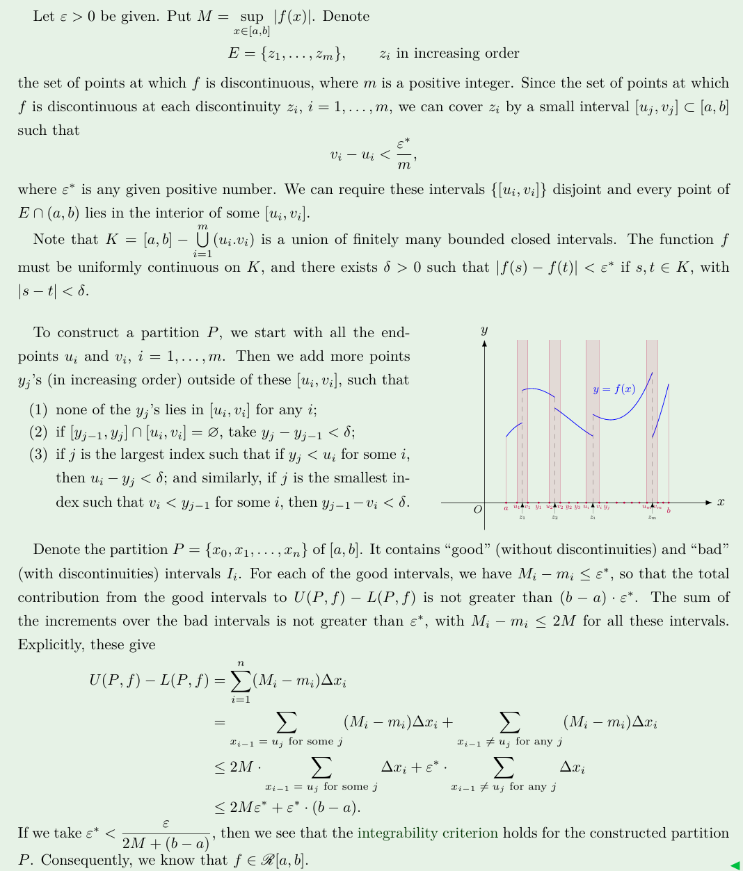
2. If \(f\) is bounded on \([a,b]\) and has only finitely many discontinuities, then \(f\in\mathscr{R}[a, b]\).

Proof Pro. 5.2.2

3. If \(f\) is monotonic on \([a, b]\), then \(f\in \mathscr{R}[a,b]\).

Proof Pro. 5.2.3

Without loss of generality, we assume that \(f\) is monotone increasing on \([a, b]\).

For any \(\epsilon >0\), we can always choose a positive interger \(n\) s.t.

\[\frac{b-a}{n}\cdot[f(b)-f(a)]<\epsilon \]

Consider a equal-spaced (等间距) partition

\[P:a=x_0<x_1<\cdots<x_{n-1}<x_n=b \]

s.t., for \(i=0, 1, \cdots, n\)

\[\Delta x_i=x_i-x_{i-1}=\frac{b-a}{n} \]

Since \(f\) is monotone increasing on \([a, b]\), we know

\[M_i=f(x_i), m_i=f(x_{i-1}) \]

Hence,

\[\begin{aligned} U(P, f)-L(P, f)&=\sum_{i=1}^n(M_i-m_i)\Delta x_i\\\\ &=\sum_{i=1}^n[f(x_i)-f(x_{i-1})]\cdot \frac{b-a}{n}\\\\ &=[f(b)-f(a)]\cdot\frac{b-a}{n}<\epsilon \end{aligned} \]

Hence, \(f\in\mathscr{R}[a, b]\).

4. If \(f\in\mathscr{R}[a, b]\), then \(f\) is bounded on \([a, b]\).

Proof Pro. 5.2.4

Suppose \(f\) is unbounded on \([a, b]\).

For any \(\epsilon >0\), for any partition \(P:a=x_0<x_1<\cdots<x_{n-1}<x_n=b\), there must exists \(p\in\{1, 2, \cdots, n\}\) s.t. \(f\) is unbouned on \([x_{p-1}, x_p]\).

Thus for any chosen \(s_p\in[x_{p-1}, x_p]\), there exists \(t_p\in[x_{p-1}, x_p]\) s.t.

\[|f(s_p)-f(t_p)|\geq \frac{\epsilon}{\Delta x_p} \]

This gives

\[\sum_{i=1}^n|f(s_i)-f(t_i)|\Delta x_i\geq |f(s_p)-f(t_p)|\Delta x_p\geq \epsilon \]

so that Condition 1 for integrability fails.

Pro. 5.3 Riemann integrability of composition

Suppose \(f\in \mathscr{R}[a, b]\), \(m\leq f\leq M\), \(\phi\) is continuous on \([m, M]\), and \(h(x)=\phi(f(x))\) on \([a, b]\). Then \(h\in\mathscr{R}[a, b]\).

Proof Pro. 5.3

Since \(\phi\) is uniformly continuous on \([m, M]\), for any given positive number \(\epsilon^*\), there exists \(\delta>0\) s.t. \(\delta<\epsilon^*\) and \(|\phi(s)-\phi(t)|<\epsilon^*\) if \(s, t\in[m, M]\), with \(|s-t|<\delta\).

Since \(f\in\mathscr{R}[a, b]\), there is a partition \(P=\{x_0, \cdots, x_n\}\) of \([a, b]\) s.t.

\[U(P, f)-L(P, f)<\delta^2 \]

Let \(M_i, m_i\) be the supremum and infimum of \(f\) on \([x_{i-1}, x_i]\), respectively, while \(M_i^*, m_i^*\) be the analogous numbers for \(h\). Divide the set \(\{1, 2, \cdots, n\}\) into two sets \(A\) and \(B\): \(i\in A\) if \(M_i-m_i<\delta\), \(i\in B\) if \(M_i-m_i\geq \delta\).

For \(i\in A\), the choice of \(\delta\) shows that \(M_i^*-m_i^*\leq \epsilon^*\).

For \(i\in B\), \(M_i^*-m_i^*\leq 2K\), where \(K=\sup_{m\leq t\leq M}|\phi(t)|\).

From

\[\delta\sum_{i\in B}\Delta x_i\leq \sum_{i\in B}(M_i-m_i)\Delta x_i\leq U(P, f)-L(P, f)<\delta^2 \]

we have

\[\sum_{i\in B}\Delta x_i<\delta \]

Thus

\[\begin{aligned} U(P, h)-L(P, h)&=\sum_{i\in A}(M_i^*-m_i^*)\Delta x_i+\sum_{i\in B}(M_i^*-m_i^*)\Delta x_i\\\\ &\leq \epsilon^*(b-a)+2K\delta\\\\ &\leq (b-a+2K)\epsilon^* \end{aligned} \]

If we take \(\epsilon^*<\frac{\epsilon}{b-a+2K}\), then we see that integrability criterion holds for the partition \(P\).

Consequently, we know that \(h\in\mathscr{R}[a, b]\).

Pro. 5.4 Properties of the Riemann Integral

1. Linearity (线性): If \(f, g\in \mathscr{R}[a, b]\) and \(\alpha, \beta\) are real numbers, then \(\alpha f+\beta g\in \mathscr{R}[a, b]\) and

\[\int_{a}^b(\alpha f+\beta g)\text{d} x=\alpha\int_{a}^{b} f\text{d} x+\beta\int_{a}^{b}g\text{d} x \]

2. Additivity (可加性): If \(f\in \mathscr{R}[a, b]\) and if \(a<c<b\), then \(f\in\mathscr{R}[a, c]\) and \(f\in\mathscr{R}[c, b]\), and

\[\int_{a}^c f\text{d}x+\int_{c}^b f\text{d}x=\int_{a}^b f\text{d}x \]

3. Monotonicity (单调性): If \(f, g\in\mathscr{R}[a, b]\), and \(f(x)\leq g(x)\), then

\[\int_{a}^{b}f\text{d}x\leq \int_{a}^{b}g\text{d}x \]

Corollary 5.4.3.1

If \(f\in\mathscr{R}[a, b]\), then \(|f|\in\mathscr{R}[a, b]\) and

\[\left|\int_{a}^bf\text{d} x\right|\leq\int_{a}^{b}|f|\text{d}x\leq M(b-a) \]

where \(|f(x)|\leq M\) on \([a, b]\).

Pro. 5.5 Mean Value Theorem for integrals (积分中值定理)

If \(f\) is continuous on \([a, b]\), then there exists a number \(c\) in \([a, b]\) such that

\[\int_{a}^{b}f(x)\text{d}x=f(c)(b-a) \]

• The fomula \(\frac{1}{b-a}\int_{a}^b f(x)\text{d}x\) gives the average value (均值) of \(f\) on \([a, b]\), and denote it as \(f_{ave}\).

Proof Pro. 5.5

According to Lagrange's Extreme Value Theorem (EVT), \(f\) must have a global maximum and global minimum.

Define \(m\triangleq\min_{x\in[a, b]}f(x), M\triangleq\max_{x\in[a, b]}f(x)\), and there exist \(x_1, x_2\) s.t. \(f(x_1)=m, f(x_2)=M\)

According to the Pro. 5.4.3, we have

\[m(b-a)\leq\int_{a}^{b}f(x)\text{d}x\leq M(b-a) \]

Thus we have

\[m\leq \frac{\int_{a}^{b}f(x)}{b-a}\leq M \]

Define \(S:=\{x|f(x)\leq \frac{\int_{a}^{b}f(x)}{b-a}, x\in[x_1, x_2]\}\).

According to the Completeness Axiom, \(\sup S\) exists, denote \(c\triangleq\sup S\).

Because \(S\subseteq [x_1, x_2], c\leq \max\{x_1, x_2\}\).

If \(f(c)< \frac{\int_{a}^{b}f(x)}{b-a}\), because of the continuity, for \(\epsilon=\frac{\int_{a}^{b}f(x)}{b-a}-f(c)>0\), exists \(\delta>0\), s.t. \(\forall x\in[x_1, x_2]\text{ and } |x-c|<\delta, |f(x)-f(c)|<\epsilon\). This implies \(\forall x\in(c-\delta, c+\delta)\cap[x_1, x_2], f(x)<\frac{\int_{a}^{b}f(x)}{b-a}\). This shows \(c+\delta\) is also the supermum of \(S\), which is in contradictory with \(c=\sup S\).

Similarly, we can prove that \(f(c)>\frac{\int_{a}^{b}f(x)}{b-a}\) does not hold.

(comment: Intermediate Value Theorem).

Thus, there exists \(c\in[x_1, x_2]\subseteq[a, b]\), s.t. \(f(c)=\frac{\int_{a}^{b}f(x)}{b-a}\).

Theo. 5.6 Fundamental Theorem of Calculus (微积分基本定理)

Part 1

Suppose \(f\in\mathscr{R}[a, b]\). For \(a\leq x\leq b\), put

\[F(x)=\int_{a}^xf(t)\text{d} t \]

Then \(F\) is continuous on \([a, b]\). Furthermore, if \(f\) is continuous at a point \(x_0\in[a, b]\), then \(F\) is differentiable at \(x_0\), and \(F^\prime(x_0)=f(x_0)\).

Proof Pro. 5.6 Part 1

Since \(f\in\mathscr{R}[a, b]\), \(f\) is bounded on \([a, b]\). Suppose \(|f(x)|\leq M, \forall x\in[a, b]\), we have

\[\forall x,y\in[a, b], |F(y)-F(x)|=|\int_{x}^yf(t)\text{d}t|\leq M|(y-x)| \]

This shows that \(f\) is uniformly continuous on \([a, b]\), thus \(f\) is continuous on \([a, b]\).

If \(f\) is continuous at \(x_0\), then for any \(\epsilon>0\), there exists \(\delta>0\) s.t.

\[\forall |x-x_0|<\epsilon \text{ and } x\in[a, b], |f(x)-f(x_0)|<\epsilon \]

Hence, if \(x_0-\delta<s\leq x_0\) and \(a\leq s\), we have

\[\begin{aligned} \left|\frac{F(x_0)-F(s)}{x_0-s}-f(x_0)\right|&=\left|\frac{1}{x_0-s}\int_{s}^{x_0}[f(u)-f(x_0)]\text{d}u\right|\\\\ &\leq \frac{1}{x_0-s}\int_{s}^{x_0}|f(u)-f(x_0)|\text{d}u\\\\ &<\frac{1}{x_0-s}\epsilon(x_0-s)=\epsilon \end{aligned} \]

Thus \(F^{\prime}_{-}(x_0)=\lim_{h\rightarrow 0^-}\frac{F(x_0+h)-F(x_0)}{h}=f(x_0)\)

Similarly, we can obtain \(F^{\prime}_{+}(x_0)=\lim_{h\rightarrow 0^+}\frac{F(x_0+h)-F(x_0)}{h}=f(x_0)\)

Thus \(F^\prime(x_0)=f(x_0)\)

Part 2

If \(f\) is continuous on \([a, b]\), and if there is a differentiable function \(F\) on \([a, b]\) such that \(F^\prime=f\), then the Newton-Leibniz formula (牛顿-莱布尼茨公式) holds:

\[\int_{a}^bf(x)\text{d}x=F(b)-F(a) \]

• A differentaible function \(F\) is called an antiderivative (反导数) of \(f\) if \(F^\prime(x)=f(x)\).

Proof Pro. 5.6 Part 2

For each given \(\epsilon>0\), there exists a partition \(P=\{x_0, \cdots, x_n\}\) of \([a, b]\), such that

\[U(P, f)-L(P, f)<\epsilon \]

For each \(i, i\in\{1, \cdots, n\}\), by the Mean Value Theorem, there is \(t_i\in[x_{i-1}, x_i]\) such that

\[F(x_i)-F(x_{i-1})=f(t_i)\Delta x_i \]

Thus

\[\sum_{i=1}^n f(t_i)\Delta x_i=F(b)-F(a) \]

According to Theo. 5.3, if the integrability criterion holds for the partition \(P\), then the same partition \(P\) is valid for Condition 2. Thus

\[\left|\sum_{i=1}^nf(t_i)\Delta x_i-\int_{a}^bf(x)\text{d}x\right|<\epsilon \]

That is,

\[\left|F(b)-F(a)-\int_{a}^bf(x)\text{d}x\right|<\epsilon \]

Since \(\epsilon\) is arbitrary, we can obtain \(\int_{a}^bf(x)\text{d}x=F(b)-F(a)\)

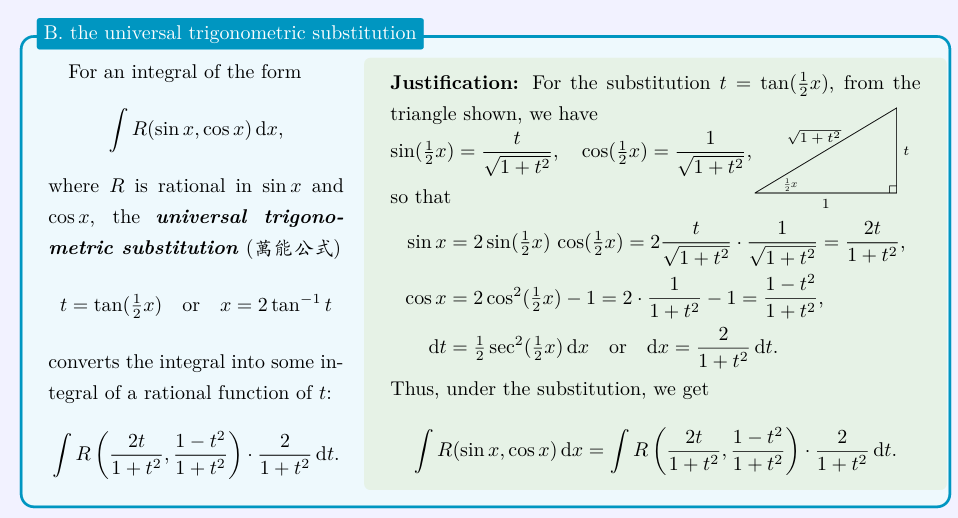
Theo. 5.7 Integration by parts and by substitution (分部积分与积分代换)

Integration by parts

Suppose \(F\) and \(G\) are differentaible functions on \([a, b]\), $F^\prime =f $ is continuous on \([a, b]\), and \(G^\prime =g\) is continuous on \([a, b]\). Then

\[\int_{a}^b F(x)g(x)\text{d}x=[F(x)G(x)]|_{x=a}^b-\int_{a}^bf(x)G(x)\text{d}x \]

Proof Pro. 5.7 Part 1

\((F(x)G(x))^\prime=F^\prime(x)G(x)+F(x)G^\prime(x)\)

\([F(x)G(x)]|_{x=a}^b=\int_{a}^b[F^\prime(x)G(x)+F(x)G^\prime(x)]\text{d}x\)

Sample 5.7 Part 1 (1)

• Calculate \(\int_{0}^{\frac{\pi}{2}}e^x\sin x\text{d}x\) and \(\int_{0}^{\frac{\pi}{2}}e^x\cos x\text{d}x\)

Let \(I=\int_{0}^{\frac{\pi}{2}}e^x\sin x\text{d}x, J=\int_{0}^{\frac{\pi}{2}}e^x\cos x\text{d}x\)

Denote \(u=\sin x, \text{d}v=e^{x}\text{d}x\), then \(\text{d}x=\cos x, v=e^{x}\)

Thus

\[\int_{0}^{\frac{\pi}{2}}e^x\sin x\text{d}x=[e^x\sin x]|_{0}^{\frac{\pi}{2}}-\int_{0}^{\frac{\pi}{2}}e^x\cos x\text{d}x \]

Thus \(I=e^{\frac{\pi}{2}}-J\).

Similarly, we can obtain

\[\int_{0}^{\frac{\pi}{2}}e^x\cos x\text{d}x=[e^x\sin x]|_{0}^{\frac{\pi}{2}}+\int_{0}^{\frac{\pi}{2}}e^x\sin x\text{d}x \]

Thus \(J=-1+I\)

Thus we can conclude

\[I=\frac{e^{\frac{\pi}{2}}+1}{2}, J=\frac{e^{\frac{\pi}{2}}-1}{2} \]

Integration by substitution

Suppose \(\phi :[a, b]\subset\mathbb R\rightarrow \mathbb R\) is differentiable and its derivative \(\phi^\prime\) is continuous on \([a, b]\). For any real continuous function \(f\) on \(\phi([a, b])\), the substitution formula holds:

\[\int_{a}^{b}f(\phi(x))\phi^\prime(x)\text{d}x=\int_{\phi(a)}^{\phi(b)}f(t)\text{d}t \]

(comment: In the context of definite integrals, the substitution function is typically required to be monotonic.)

Proof Pro. 5.7 Part 2

Since \(f\) is continuous, by Part 1 of the Fundamental Theorem of Calculus, we can define

\[F(x)=\int_{\phi(a)}^xf(t)\text{d}t \]

and have \(F^\prime(x)=f(x)\). By the hypothesis, the function \(\phi\) is differentiable, so that, by the chain rule, we have

\[[F(\phi(x))]^\prime=F^\prime(\phi(x))\cdot\phi^\prime(x)=f(\phi(x))\cdot \phi^\prime(x) \]

Since \(f\) and \(\phi\) are continuous, the composition \(f(\phi(x))\) is continuous and therefore integrable. It follows from the Newton-Leibniz formula that

\[\begin{aligned} \int_{a}^{b}f(\phi(x))\cdot\phi^\prime(x)\text{d}x&=[F(\phi(x))]|_{x=a}^b\\\\ &=F(\phi(b))-F(\phi(a))\\\\ &=\int_{\phi(a)}^{\phi(b)}f(t)\text{d}t-\int_{\phi(a)}^{\phi(a)}f(t)\text{d}t\\\\ &=\int_{\phi(a)}^{\phi(b)}f(t)\text{d}t \end{aligned} \]

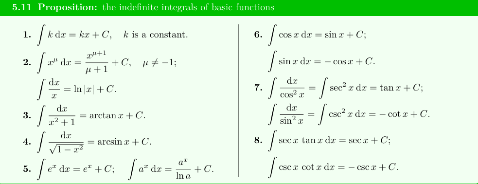
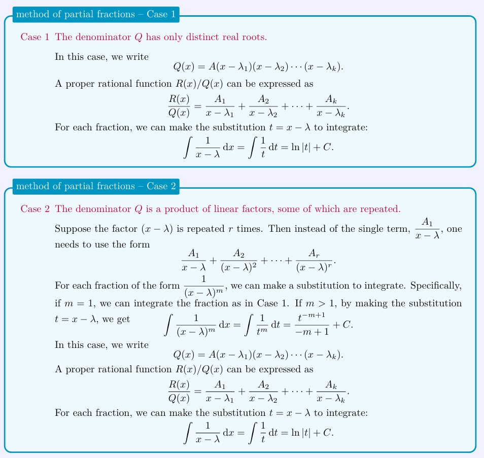
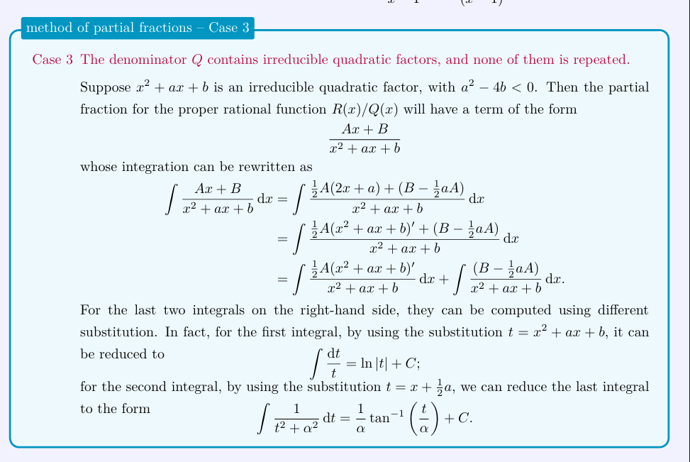
Pro. 5.8 The indefinite integrals of basic functions

Pro. 5.9 Linearity of the indefinite integral

For any two numbers \(\alpha\) and \(\beta\), the indefinite integral satisfies the linear equality

\[\int (\alpha f+\beta g)\text{d}x=\alpha\int f\text{d}x+\beta\int g\text{d}x \]

Theo. 5.10 Integration by parts and by substitution for the indefinite integral

Integration by parts

If \(f\) and \(g\) are differentiable functions, then

\[\int f(x)\text{d}g(x)=f(x)g(x)-\int g(x)\text{d}f(x) \]

Integration by substitution

If \(f\) is continuous and \(\phi\) is differentiable, then

\[\int f(\phi(x))\phi^\prime(x)\text{d}x=\left.\int f(t)\text{d}t\right|_{t=\phi(x)} \]

Theo. 5.11 Comparison Test for improper integrals (比较审敛法)

Suppose that \(f, g\in\mathscr{R}[a, t]\) for all \(t>a\) and that they satisfy \(0\leq f(x)\leq g(x)\) on \([a, \infty)\).

1. If \(\int_{a}^{\infty}g(x)\text{d}x\) converges, then \(\int_{a}^{\infty}f(x)\text{d}x\) converges.

2. If \(\int_{a}^{\infty}f(x)\text{d}x\) diverges, then \(\int_{a}^{\infty}g(x)\text{d}x\) diverges.

Coro. 5.11.1

Suppose \(f\in\mathscr{R}[a, t]\) for all \(t>a\).

1. If \(f\) satisfies \(0\leq f(x)\leq\frac{1}{x^p}\) on \([a, \infty)\) for some \(p>1\), then \(\int_{a}^{\infty} f(x)\text{d}x\) converges.

2. If \(f\) satisfies \(f(x)\geq\frac{1}{x^p}\) on \([a, \infty)\) for some \(0<p\leq 1\), then \(\int_{a}^{\infty} f(x)\text{d}x\) diverges.

Coro. 5.11.2 Limit Comparison Test for improper integrals

Suppose that \(f, g\in\mathscr{R}[a, t]\) for all \(t>a\), and that they are both non-negative on \([a, \infty)\) and satisfy

\[\lim_{x\rightarrow\infty}\frac{f(x)}{g(x)}=L \]

1. If \(L=0\), then \(\int_{a}^{\infty}f(x)\text{d}x\) converges if \(\int_{a}^{\infty}g(x)\text{d}x\) converges.

2. If \(0<L\) and \(L\) exists, then \(\int_{a}^{\infty}f(x)\text{d}x\) converges if and only if \(\int_{a}^{\infty}g(x)\text{d}x\) converges.

3. If \(L=\infty\), then \(\int_{a}^{\infty}f(x)\text{d}x\) diverges if and only if \(\int_{a}^{\infty}g(x)\text{d}x\) diverges.

Theo. 5.12 Absolute convergence of improper integrals (反常积分的绝对收敛性)

If \(\int_{a}^{\infty} |f(x)|\text{d}x\) converges, then \(\int_{a}^{\infty} f(x)\text{d}x\) also converges.

However, the converse does NOT hold.

Proof Pro. 5.12

If \(\int_{a}^{\infty}|f(x)|\text{d}x\) converges, then, by the Cauchy criterion, for every \(\epsilon>0\), there exists \(N\) s.t. for any \(t_1, t_2\geq N\),

\[\left|\int_{t_1}^{t_2}|f(x)|\text{d}x\right|<\epsilon \]

Thus, for \(t_1, t_2\geq N\) (assuming \(t_1<t_2\)), we have

\[\left| \int_{t_1}^{t_2}f(x)\text{d}x\right|\leq \int_{t_1}^{t_2}|f(x)|\text{d}x<\epsilon \]

This means that the Cauchy criterion holds for the limit \(\lim_{t\rightarrow\infty}\int_{a}^{t}f(x)\text{d}x\).

Coro. 5.12.1

Suppose \(f, h:[a, \infty]\rightarrow \mathbb R\).

• \(h\geq 0\), monotone decreasing, \(\lim_{x\rightarrow \infty}h(x)=0\)

• \(|\int_{a}^{t}f(x)\text{d}x|\leq M, \forall t\in[a, +\infty)\)

Then,

\[\int_{a}^{+\infty}f(x)h(x)\text{d}x \text{ converges} \]

Proof Coro. 5.12.1

Denote \(F(x)=\int_{a}^{x}f(u)\text{d}u\)

\[\begin{aligned} \int_{a}^{t}f(x)h(x)\text{d}x&= h(x)F(x)|_{x=a}^{t}-\int_{a}^{t}F(x)h^\prime(x)\text{d}x\\\\ &=h(t)F(t)-h(a)F(a)-\int_{a}^{t}F(x)h^\prime(x)\text{d}x\\\\ &=h(t)F(t)-\int_{a}^{t}F(x)h^\prime(x)\text{d}x\\\\ \end{aligned} \]

Since \(|F(x)|\leq M\), \(h^\prime(x)\leq 0\)

\[\begin{aligned} \int_{a}^{t}|F(x)h^\prime(x)|\text{d}x & \leq M\int_{a}^{t}|h^\prime(x)|\text{d}x\\\\ & \leq M(h(a)-h(t))\\\\ \end{aligned} \]

Thus for any \(\epsilon>0\), \(\exists N>0\) s.t. \(\forall t>N\), \(\left|\int_{a}^{t}|F(x)h^\prime(x)|\text{d}x-Mh(a)\right|\leq Mh(t)<\epsilon\).

Thus \(\int_{a}^{t}|F(x)h^\prime(x)|\text{d}x\) converges. Then from Theo. 5.12, \(\int_{a}^{t}F(x)h^\prime(x)\text{d}x\) also converges.

Since \(h(t)\) and \(F(t)\) also converges when \(t\rightarrow \infty\), we can obtain \(\int_{a}^{+\infty}f(x)h(x)\text{d}x\) converges.

Method

Indefinite Integral

Numerical Approximations (数值近似)

Trapezoidal rule (梯形法) & Midpoint rule (中点法)

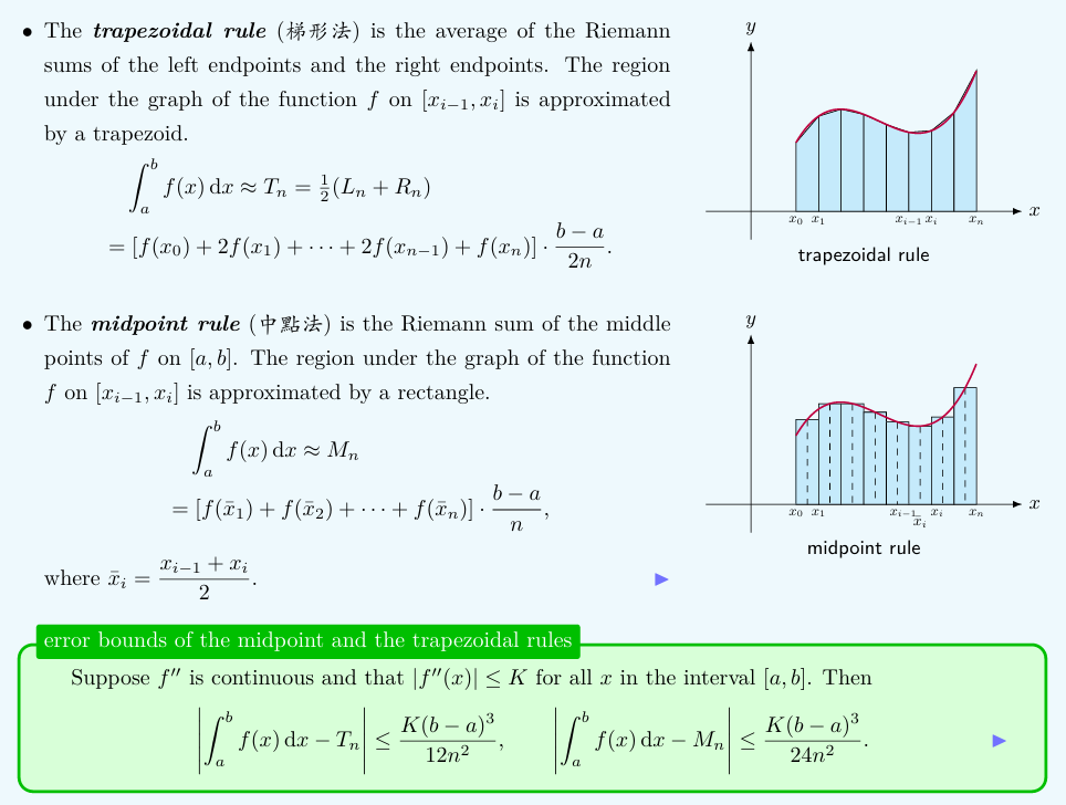
Proof: error bound of the midpoint rule

\(g(h)\triangleq \int_{0}^hf\text{d}x-\frac{h(f(0)+f(h))}{2}\)

\(g^\prime(h)=f(h)-\frac{f^\prime(h)\cdot h}{2}-\frac{f(0)+f(h)}{2}=\frac{f(0)-f(h)}{2}-\frac{f^\prime(h)\cdot h}{2}\)

\(g^{\prime\prime}(h)=-\frac{f^{\prime\prime}(h)\cdot h}{2}\)

\(g^\prime(r)=g^\prime(0)+\int_{0}^r g^{\prime\prime}(t)\text{d}t=\int_{0}^r g^{\prime\prime}(t)\text{d}t\)

\[\begin{aligned} g(h)&=g(0)+\int_{0}^h g^\prime(r)\text{d}r\\\\ &=\int_{0}^h\int_{0}^rg^{\prime\prime(t)}\text{d}t\text{d}r\\\\ \end{aligned} \]

\[\begin{aligned} |g(h)|&\leq \int_{0}^h\left|\int_{0}^rg^{\prime\prime(t)}\text{d}t\right|\text{d}t\\\\ &\leq \int_{0}^h\int_{0}^r\left|g^{\prime\prime(t)}\right|\text{d}t\text{d}t\\\\ &\leq \int_{0}^h\int_{0}^r\frac{K}{2}h\text{d}t\text{d}t\\\\ &=\frac{K}{2}\int_{0}^h\frac{t^2}{2}|_{t=0}^r\text{d}r\\\\ &=\frac{K}{4}\frac{r^3}{3}|_{r=0}^h=\frac{K}{12}h^3 \end{aligned} \]

Proof: error bound of the trapezoidal rule

Take \(c=\frac{h}{2}\)

By Taylor expansion

\[f(x)=f(c)+f^\prime(c)(x-c)+\frac{f^{\prime\prime}(\theta_x)}{2}(x-c)^2 \]

for some \(\theta_x\in[0, x]\).

Thus,

\[\begin{aligned} \left|\int_{0}^hf(x)\text{d}x-f(c)\cdot h\right| &\leq \frac{K}{2}\int_{0}^h (x-\frac{h}{2})^2\text{d}x\\\\ &=\frac{K}{6}(x-\frac{h}{2})^3|_{x=0}^h=\frac{K}{24}h^3 \end{aligned} \]

Properties of the error bounds:

• trade-off between cost & accuracy

• round off error, not accounted

• neat, i.e. explicit constant & non-asymptotic

• If only \(f^\prime\) is continuous, all these rules has accuracy \(\sim O(\frac{1}{n})\)

• curse of dimensionality

• Monte-Carlo tackles curse of dimensionality

[csdn] 蒙特卡罗(Monte Carlo)方法简介 - wuguangbin1230

(Week) Law of Large Number

\(Z_1, \cdots, Z_M \stackrel{i.i.d.}{\sim} \text{distr.}\)

\(\bar{Z}=\frac{1}{M}\sum_{i=1}^{M}Z_i\)

\(\mathbb {E}[\bar{Z}]=\frac{\mathbb{E}[Z_1]}{M}\)

\(\text{VAR}[\bar{Z}]=\frac{\text{VAR}[Z_1]}{M}\)

\(\left|\frac{\sum_{1}^iZ_i}{M}-\mathbb{E}[Z_1]\right|\sim O(\frac{1}{\sqrt M})\) with high probability.

\(U\sim \text{Uni} f[0,1]^d, Z\triangleq f(U)\)

\[\mathbb{E}[Z]=\int_{[0, 1]^d}f(x)\text{d}x \]

Simpson's rule for the numerical approximation of integrals (辛普森法)

Let \(f\) be an integrable function over \([a, b]\). For an even integer \(n\), divide the interval \([a, b]\) into \(n\) subintervals of equal length:

\[x_0=a, x_1=a+\frac{b-a}{n}, \cdots, x_{n-1}=a+\frac{(n-1)(b-a)}{n}, x_{n}=b \]

Simpson's rule is the approximation to \(\int_{a}^{b}f\text{d}x\):

\[\begin{aligned} \int_{a}^{b}f\text{d}x\approx\frac{b-a}{3n}[f(x_0)+4f(x_1)+2f(x_2)+4f(x_3)+\cdots+2f(x_{n-2})+4f(x_{n-1})+f(x_n)] \end{aligned} \]

Error bound of Simpson's rule:

\[|\int_{a}^bf(x)\text{d}x-S_n|\leq \frac{K(b-a)^5}{180n^4} \]

Others

Irrationality of \(\pi\) (Ivan Niven 1947)

Suppose \(\pi=\frac{p}{q}\), for som \(p, q\in \mathbb {N}\).

\(f(x)\triangleq\frac{x^n(p-qx)^n}{n!}\)

\(I\triangleq \int_{0}^{\pi} f(x)\sin x\text{d}x\)

\[\begin{aligned} I&=-\int_{0}^{\pi}f(x)\text{d}\cos x\\\\ &=(-\cos xf(x))|_{x=0}^{\pi}+\int_{0}^{\pi}f^{(1)}(x)\cos x\text{d}x\\\\ &=\text{integer}+(f^{(1)}(x)\sin x)|_{x=0}^{\pi}-\int_{0}^{\pi}f^{(2)}(x)\sin x\text{d}x\\\\ &=\cdots\\\\ &=\text{integer} \end{aligned} \]

note that \(\max f(x)\) is attained at \(x^{*}=\frac{\left(\frac{p}{2}\right)^{2n}}{n!}\)

Thus \(0<I\leq f(x^{*})=\frac{\left(\frac{p}{2}\right)^{2n}}{n!}\stackrel{n \text{ is large enough}}{<} 1\), which conflicts with \(I\in N_{0}\)

Taylor expansion of \(\pi\)

\(\arctan(x)=\sum_{k=0}^{\infty}\frac{(-1)^kx^{2k+1}}{2k+1}\)

\(\arctan(1)=\frac{\pi}{4}\)

Approximate \(\pi\) with Monte-Carlo

\[\frac{|\lbrace X|X \in \text{Circle}\rbrace|}{|X|}\stackrel{\text{LLN}}{\approx}\frac{\pi}{4} \]

\(\pi\approx \frac{22}{7}\)

\[\begin{aligned} \int_{0}^{1}\frac{u^4(1-u)^4}{1+u^2}\text{d}u&=\int_{0}^{1}(u^6-4u^5+5u^4-4u^2+4)\text{d}u-4\int_{0}^{1}\frac{1}{1+u^2}\text{d}u\\\\ &=\frac{22}{7}-4(\arctan u)|_{u=0}^{1}\\\\ &=\frac{22}{7}-\pi \end{aligned} \]

\[\int_{0}^{1}\frac{u^4(1-u)^4}{1+u^2}\text{d}u<\int_{0}^{1}u^4(1-u)^4\text{d}u=\frac{1}{630} \]

\[\int_{0}^{1}\frac{u^4(1-u)^4}{1+u^2}\text{d}u>\int_{0}^{1}\frac{u^4(1-u)^4}{2}\text{d}u=\frac{1}{1260} \]

Thus

\[\frac{1}{1260}<\frac{22}{7}-\pi<\frac{1}{630} \]

Taylor expansion

Assuming \(f\in \mathscr{D}^{n+1} (I), a\in I\).

\[\begin{aligned} f(x)&=f(a)+\int_{a}^{x}f^{(1)}(x_1)\text{d}x_1\\\\ f^{(1)}(x)&=f^{(1)}(a)+\int_{a}^{x}f^{(2)}(x_2)\text{d}x_2\\\\ f^{(2)}(x)&=f^{(2)}(a)+\int_{a}^{x}f^{(3)}(x_3)\text{d}x_3\\\\ &\vdots\\\\ f^{(n)}(x)&=f^{(n)}(a)+\int_{a}^{x}f^{(n+1)}(x_{n+1})\text{d}x_{n+1}\\\\ \end{aligned} \]

\[\begin{aligned} f(x)&=f(a)+\int_{a}^{x}f^{(1)}(x_1)\text{d}x_1\\\\ &=f(a)+\int_{a}^{x}f^{(1)}(a)\text{d}x_{1}+\int_{a}^{x}\int_{a}^{x_1}f^{(2)}(x_2)\text{d}x_{2}\text{d}_{x_1}\\\\ &=\cdots\\\\ &=f(a)+\int_{a}^{x}f^{(1)}(a)\text{d}x_{1}+\int_{a}^{x}\int_{a}^{x_1}f^{(2)}(a)\text{d}x_{2}\text{d}_{x_1}+\cdots+\int_{a}^{x}\int_{a}^{x_1}\cdots\int_{a}^{x_{n-1}}f^{(n)}(a)\text{d}x_{n}\text{d}x_{n}\cdots \text{d}x_{2}\text{d}x_{1}+\int_{a}^{x}\int_{a}^{x_1}\cdots\int_{a}^{x_{n}}f^{(n+1)}(a)\text{d}x_{n+1}\text{d}x_{n}\cdots \text{d}x_{2}\text{d}x_{1}\\\\ &= f(a)+f^{(1)}(a)(x-a)+f^{(2)}(a)\frac{(x-a)^2}{2}+\cdots+f^{(n)}(a)\frac{(x-a)^n}{n!}+\#\frac{(x-a)^{n+1}}{(n+1)!} & (\forall x\in[a, x_{n}],m\leq f^{(n+1)}(x)\geq K, \#\in[m, M])\\\\ &=f(a)+f^{(1)}(a)(x-a)+f^{(2)}(a)\frac{(x-a)^2}{2}+\cdots+f^{(n)}(a)\frac{(x-a)^n}{n!}+o(\frac{1}{n!}) \end{aligned} \]

\[\begin{aligned} I_n&\triangleq\int_{a}^{x}(x-t)^nf^{(n+1)}(t)\text{d}t\\\\ &=(x-t)^nf^{(n)}(t)|_{t=a}^{x}+n\int_{a}^{x}(x-t)^{n-1}f^{(n)}(t)\text{d}t & (\text{Integration by parts})\\\\ &=-(x-a)^nf^{(n)}(a)+nI_{n-1}\\\\ &=-\left((x-a)^nf^{(n)}(a)+n(x-a)^{n-1}f^{(n-1)}+\cdots+n(n-1)\cdots(2)(x-a)f^{(1)}(a)\right)+n!\left(f(x)-f(a)\right)\\\\ \end{aligned} \]

\[f(x)=\sum_{k=0}^n\frac{f^{(k)}(a)(x-a)^k}{k!}+\frac{I_n}{n!} \]

• Cauthy Form

  • by MVT, \(I_n=(x-a)(x-\theta)^nf^{(n+1)}(\theta)\) for some \(\theta\in[a, x]\)

• Lagrange Form

  • EMVT: \(f:I\rightarrow\mathbb{R}\), cont. on \(I\), \(\phi:I\rightarrow\mathbb{R}, \phi\geq 0\), integrable on \(I\) \(\Rightarrow\) \(\int_{a}^{b}f(t)\phi(t)\text{d}t=f(\theta)\int_{a}^{b}\phi(t)\text{d}t\) for some \(\theta\in I\).
  • by EMVT, \(I_n=f^{(n+1)}(\theta)\int_{a}^{x}(x-t)^n\text{d}t=f^{(n+1)}(\theta)\cdot\frac{(x-a)^{n+1}}{n+1}\) for some \(\theta\in [a, x]\)

Cauthy Distribution

PDF:

\[f_{X}(x)=\frac{1}{\pi(1+x^2)} \]

\[\begin{aligned} \int_{-\infty}^{\infty}f_{X}(x)&=\int_{-\infty}^{\infty}\frac{1}{\pi(1+x^2)}\\\\ &=\int_{-\infty}^{0}\frac{1}{\pi(1+x^2)}+\int_{0}^{\infty}\frac{1}{\pi(1+x^2)}\\\\ &=\frac{1}{\pi}\cdot\frac{\pi}{2}+\frac{1}{\pi}\cdot\frac{\pi}{2}\\\\ &=1 \end{aligned} \]

\[\begin{aligned} E[X]&=\int_{-\infty}^{\infty}xf_{X}(x)\\\\ &=\int_{-\infty}^{\infty}\frac{x}{\pi(1+x^2)}\\\\ &=\int_{-\infty}^{0}\frac{x}{\pi(1+x^2)}+\int_{0}^{\infty}\frac{x}{\pi(1+x^2)}\\\\ \end{aligned} \]

Since \(\int_{0}^{\infty}\frac{x}{\pi(1+x^2)}=\frac{\lim_{t\rightarrow \infty} \ln t}{\pi}\) diverges, \(E[X]\) does not exist.

Euler's Formular

\[e^{ix}=\cos x+i\sin x \]

Proof

According to Taylor expansion:

\[e^z=\sum_{k=0}^\infty\frac{z^k}{k!} \]

\[\sin x=\sum_{k=0}^\infty \frac{x^{2k+1}(-1)^k}{(2k+1)!} \]

\[\cos x=\sum_{k=0}^\infty \frac{x^{2k}(-1)^k}{(2k)!} \]

Thus

\[\begin{aligned} e^{ix}&=\sum_{k=0}^\infty\frac{i^kx^k}{k!}\\\\ &=\cos x+i\sin x \end{aligned} \]

Sample 1

• \(\sin(x+y)=\sin x\cos y+\cos x\sin y\)

• \(\cos(x+y)=\cos x\cos y-\sin x\sin y\)

\[\begin{aligned} \cos(x+y)+i\sin(x+y)&=e^{i(x+y)}\\\\ &=e^{ix}\cdot e^{iy}\\\\ &=(\cos x+i\sin x)\cdot(\cos y+i\sin y)\\\\ &=\cos x\cos y-\sin x\sin y+i(\sin x\cos y+\cos x\sin y) \end{aligned} \]

Sample 2

Find \(\sum_{k=1}^n \sin(kx)\)

Solution

\[\begin{aligned} \sum_{k=1}^n \sin(kx)&=\Im(\sum_{k=1}^ne^{ikn})\\\\ &=\Im(\frac{e^{(n+1)ix}-e^{ix}}{e^{ix}-1})\\\\ &=\Im(\frac{\lbrace\cos[(n+1)x]-\cos x\rbrace+i\lbrace\sin[(n+1)x]-\sin x\rbrace}{\cos x-1+i\sin x})\\\\ &=\frac{\lbrace\sin[(n+1)x]-\sin x\rbrace(\cos x-1)-\lbrace\cos[(n+1)x]-\cos x\rbrace\sin x}{(\cos x-1)^2+\sin^2 x}\\\\ &=\frac{-\sin[(n+1)x]+\sin (nx)+\sin x}{2-2\cos x} \end{aligned} \]

Integration in machine learning

Goal: Want to learn PDF \(p_{0}(\xi)\) from samples \((X_1, X_2, \cdots, X_m)\) with a parameter model \(p_{\theta}(\xi)\).

Assumption:

• \(\lim_{\xi\rightarrow \pm\infty}p_{0}(\xi)=0\).

• \(\psi_{0}, \psi_{\theta}, \psi_{\theta}^{\prime}\) are bounded for any \(\theta\).

• \(\text{support } \psi_{\theta}\subseteq\text{support } p_{0}\)

• \(\text{support } p_{\theta}\subseteq\text{support } p_{0}\)

  • \(\text{support } h\triangleq \lbrace x\in\mathbb{R}|h(x)\neq 0\rbrace\)

Define objective function (目标函数) \(J(\theta)\):

\[J(\theta)\triangleq \int_{-\infty}^{+\infty}p_{0}(\xi)\left(\psi_{\theta}(\xi)-\psi_{0}(\xi)\right)^2\text{d}\xi \]

where \(\psi_{0}(\xi)\triangleq\frac{\text{d}}{\text{d}\xi}\ln p_{0}(\xi), \psi_{\theta}(\xi)\triangleq\frac{\text{d}}{\text{d}\xi}\ln p_{\theta}(\xi)\)

• Lemma 1:

  • If \(J(\theta^{*})=0\) for some \(\theta^{*}\), then \(\psi_{\theta^{*}}(\xi)=\psi_{0}(\xi)\) for any \(\xi \in \text{support } p_0\)

  • Proof:

    • By assumption, \(\log p_{\theta^{*}}(\xi)=\log p_{0}(\xi)+C\)

    • \(\because 1=\int_{-\infty}^{\infty}p_{\theta^{*}}(\xi)\text{d}\xi=e^C\cdot \int_{-\infty}^{\infty}p_{0}(\xi)\text{d}\xi=e^C\)

    • \(\therefore C=0\)

\[J(\theta)=\int_{-\infty}^{+\infty}p_{0}(\xi)\left(\psi_{\theta}(\xi)^2-2\psi_{\theta}(\xi)\psi_{0}(\xi)+\psi_{0}(\xi)^2\right)\text{d}\xi \]

\(\psi_{\theta}(\xi)\) is known, and \(p_{0}(\xi)\) can be obtained by Monte-Carlo.

Since it is hard to obtain \(\psi_{0}(\xi)\), we should try to avoid calculating \(\psi_{0}(\xi)\).

Since for any \(\theta\), \(J(\theta)\) always contains \(\int_{-\infty}^{+\infty}p_{0}(\xi)\psi_{0}(\xi)^2\text{d}\xi\), we don't need to consider this one.

Thus we only need to consider \(\int_{-\infty}^{+\infty}p_{0}(\xi)\psi_{\theta}(\xi)\psi_{0}(\xi)\text{d}\xi\).

\[\begin{aligned} &\int_{-\infty}^{+\infty}p_{0}(\xi)\psi_{\theta}(\xi)\psi_{0}(\xi)\text{d}\xi\\\\ &=\int_{-\infty}^{+\infty}p_{0}(\xi)\psi_{\theta}(\xi)\text{d}\ln p_{0}(\xi)\\\\ &=\int_{-\infty}^{+\infty}p_{0}(\xi)\psi_{\theta}(\xi)\cdot\frac{1}{p_{0}(\xi)}p_{0}^\prime(\xi)\\\\ &=\int_{-\infty}^{+\infty}\psi_{\theta}(\xi)p_{0}^\prime(\xi)\\\\ &=(\psi_{\theta}(\xi)p_{0}(\xi))|_{\xi=-\infty}^{+\infty}-\int_{-\infty}^{+\infty}\psi_{\theta}^\prime(\xi)p_{0}(\xi)\\\\ \end{aligned} \]

Thus

\[\widetilde{J}(\theta)\triangleq \int_{-\infty}^{+\infty}p_{0}(\xi)\left(\psi_{\theta}(\xi)^2-2\psi_{\theta}(\xi)\psi_{0}(\xi)\right)\text{d}\xi=\int_{-\infty}^{+\infty}p_{0}(\xi)\left(\psi_{\theta}(\xi)^2+2\psi^\prime_{\theta}(\xi)\right)\text{d}\xi \]

Dirichlet test

Given \(f, g: \mathbb{R}\rightarrow \mathbb{R}\).

• \(g\geq 0\), monotone decreasing, \(\lim_{x\rightarrow \infty}g(x)=0\)

• \(\exists M>0\), s.t. \(|\int_{0}^{t}f(x)\text{d}x|\leq M\) for any \(t>0\)

Then

\[\int_{0}^{\infty}f(x)g(x)\text{d}x\text{ converges.} \]

Proof

• Firstly assume \(g^\prime\) converges.

\[\begin{aligned} F(t)\triangleq \int_{0}^{t}f(x)\text{d}x \end{aligned} \]

\[\begin{aligned} \int_{0}^{t}f(x)g(x)\text{d}x&=\int_{0}^{t}g(x)\text{d}F(x)\\\\ &=g(x)F(x)|_{x=0}^{t}-\int_{0}^{t}F(x)g^\prime(x)\text{d}x \end{aligned} \]

Since \(|g(x)F(x)|\leq |g(x)||F(x)|\leq |g(x)|M\stackrel{x\rightarrow \infty}{\longrightarrow} 0\)

Thus \(g(x)F(x)|_{x=0}^{t}\) converges.

Using Cauchy critetion.

\[\begin{aligned} \int_{t_1}^{t_2}F(x)g^\prime(x)\text{d}x&=F(\theta_{t_1, t_2})\int_{t_1}^{t_2}g^\prime(x)\text{d}x & (\text{EMVT})\\\\ &\leq M|g(t_2)-g(t_1)| \end{aligned} \]

Since \(\forall \epsilon>0, \exists N>0\) s.t. for any \(t_1, t_2>N\), \(|g(t_1)-g(t_2)|<\frac{\epsilon}{M}\).

Thus \(\forall \epsilon>0, \exists N>0\) s.t. for any \(t_1, t_2>N\), \(\int_{t_1}^{t_2}F(x)g^\prime(x)\text{d}x\leq M|g(t_2)-g(t_1)|<\epsilon\)

Thus \(\int_{0}^{\infty}F(x)g^\prime(x)\text{d}x\) also converges.

Thus \(\int_{0}^{t}f(x)g(x)\text{d}x\) converges.

• Then assuming \(g\) may not be differentiable on \(\mathbb{R}\)

Using convolution to approximate.

use \(\phi_n\) s.t. \(\phi_n^\prime\) continuous, \(\text{support} \phi_n, \phi_n^{\prime}\subseteq [-\frac{1}{n}, \frac{1}{n}]\)

Suppose \(\int_{-\infty}^{\infty}\phi_{n}=1\) and \(\phi_{n}\) is non-negative.

Observation:

\[[\phi_n*g](x)=\int_{-\infty}^{\infty}g(z)\phi_n(z-x)\text{d}z \]

is monotone decreasing and has contiuous derivative.

\[[\phi_n*g]^\prime(x)=\int_{-\infty}^{\infty}g(z)\phi_n^\prime(z-x)\text{d}z \]

By the previous part, we can obtain \(\int_{0}^{\infty}\phi_n*g \cdot f\) converges.

As

\[\lim_{n\rightarrow \infty}\phi_{n}(x)= \begin{cases} 1, &x=0\\\\ 0, &x\neq0 \end{cases} \]

We can approximately obtain \(\lim_{n\rightarrow \infty}\phi_{n}(x)\times g=g\) (need more work here to rigorously prove this equation).

Thus we can obtain \(\int_{0}^{\infty}g \cdot f\) converges.

eg: \(\int_{1}^{\infty}\frac{\cos x}{x}\text{d}x\)

Abel test

• \(\int_{0}^{\infty} f(x)\text{d}x\) converges.

• h is bounded and monotone

Then \(\int_{0}^{\infty} f(x)h(x)\text{d}x\) converges.

Calculation for \(\int \sqrt{t-x^2}\text{d}x\)

\(u=\arcsin(\frac{x}{\sqrt t}), \text{d}x=\sqrt{t}\cos u\text{d}u\)

\[\begin{aligned} \int \sqrt{t-x^2}\text{d}x&=\int\sqrt{t-t\sin^2u}\sqrt{t}\cos u\text{d}u\\\\ &=\int t\cos^2 u\text{d}u\\\\ &=t\int \frac{\cos(2u)+1}{2}\text{d}u & (\cos^2u=\frac{1+\cos 2u}{2})\\\\ &=\frac{t}{2}\cdot u+\frac{t}{2}\cdot \frac{\sin 2u}{2}+C\\\\ &=\frac{t \arcsin(\frac{x}{\sqrt t})}{2}+\frac{t\sin (2\arcsin(\frac{x}{\sqrt t}))}{4}+C\\\\ \end{aligned} \]

\(y=2\arcsin(\frac{x}{\sqrt t}), \sin (\frac{y}{2})=\frac{x}{\sqrt t}, \cos (\frac{y}{2})=\frac{\sqrt{t-x^2}}{\sqrt t}\)

\(\sin y=2\sin(\frac{y}{2})\cos(\frac{y}{2})=2\cdot \frac{x}{\sqrt t}\cdot \frac{\sqrt{t-x^2}}{\sqrt t}=\frac{2x\sqrt{t-x^2}}{t}\)

\[\int \sqrt{t-x^2}\text{d}x=\frac{t \arcsin(\frac{x}{\sqrt t})}{2}+\frac{x\sqrt{t-x^2}}{2}+C \]

Calculation for \(\int \sqrt{t+x^2}\text{d}x\)

\(u=\arctan(\frac{x}{\sqrt t}), \text{d}x=\frac{\sqrt{t}}{\cos^2 u}\text{d}u\)

\[\begin{aligned} \int \sqrt{t+x^2}\text{d}x&=\int\sqrt{t+t\tan^2 u}\frac{\sqrt{t}}{\cos^2 u}\text{d}u\\\\ &=\int \frac{t}{\cos^3 u}\text{d}u\\\\ &=t\int\sec^3u\text{d}u \end{aligned} \]

Since

\[\int \sec^n x\text{d}x=\frac{\sec^{n-2} x\tan x}{n-1}+\frac{n-2}{n-1}\int \sec^{n-2}x\text{d}x \]

(take \(p=\sec^{n-2}x\), \(q=\tan x\) and apply integration by parts.)

we can obtain

\[\begin{aligned} \int \sqrt{t+x^2}\text{d}x&=t\int\sec^3u\text{d}u\\\\ &=\frac{t\sec u\tan u}{2}+\frac{t\int \sec u\text{d}u}{2}\\\\ &=\frac{\sec u\tan u}{2}+\frac{t}{2}\int \frac{\sec u(\sec u+\tan u)}{\sec u+\tan u}\text{d}u \end{aligned} \]

\(w=\sec u+\tan u, \frac{\text{d}w}{\text{d}u}=\sec u\tan u+\sec^2\)

\[\begin{aligned} \int \sqrt{t+x^2}\text{d}x&=\frac{t\sec u\tan u}{2}+\frac{t}{2}\int \frac{\sec u(\sec u+\tan u)}{\sec u+\tan u}\text{d}u\\\\ &=\frac{t\sec u\tan u}{2}+\frac{t}{2}\int\frac{1}{w}\text{d}w\\\\ &=\frac{t\sec u\tan u}{2}+\frac{t\ln|w|}{2}+C\\\\ &=\frac{t\sec u\tan u}{2}+\frac{t\ln|\sec u+\tan u|}{2}+C\\\\ &=\frac{t\sec (\arctan(\frac{x}{\sqrt t}))\tan (\arctan(\frac{x}{\sqrt t}))}{2}+\frac{t\ln|\sec (\arctan(\frac{x}{\sqrt t}))+\tan (\arctan(\frac{x}{\sqrt t}))|}{2}+C\\\\ &=\frac{t\cdot\frac{x}{\sqrt t}\cdot \frac{\sqrt{x^2+t}}{\sqrt{t}}}{2}+\frac{t\ln|\frac{\sqrt{x^2+t}}{\sqrt{t}}+\frac{x}{\sqrt t}|}{2}+C\\\\ &=\frac{x\sqrt{x^2+t}}{2}+\frac{t\ln|\sqrt{x^2+t}+x|}{2}-\frac{t\ln|\sqrt t|}{2}+C\\\\ &=\frac{x\sqrt{x^2+t}}{2}+\frac{t\ln|\sqrt{x^2+t}+x|}{2}+C\\\\ \end{aligned} \]