第二次作业：卷积神经网络 part 1

一、视频学习及问题总结

• 深度学习的数学基础

1.1 矩阵线性变换

给定的矩阵A，假设其特征值为λ，特征向量为x，则有Ax=λx ， 特征向量只有尺度变化，没有方向变化，变化系数就是特征值。

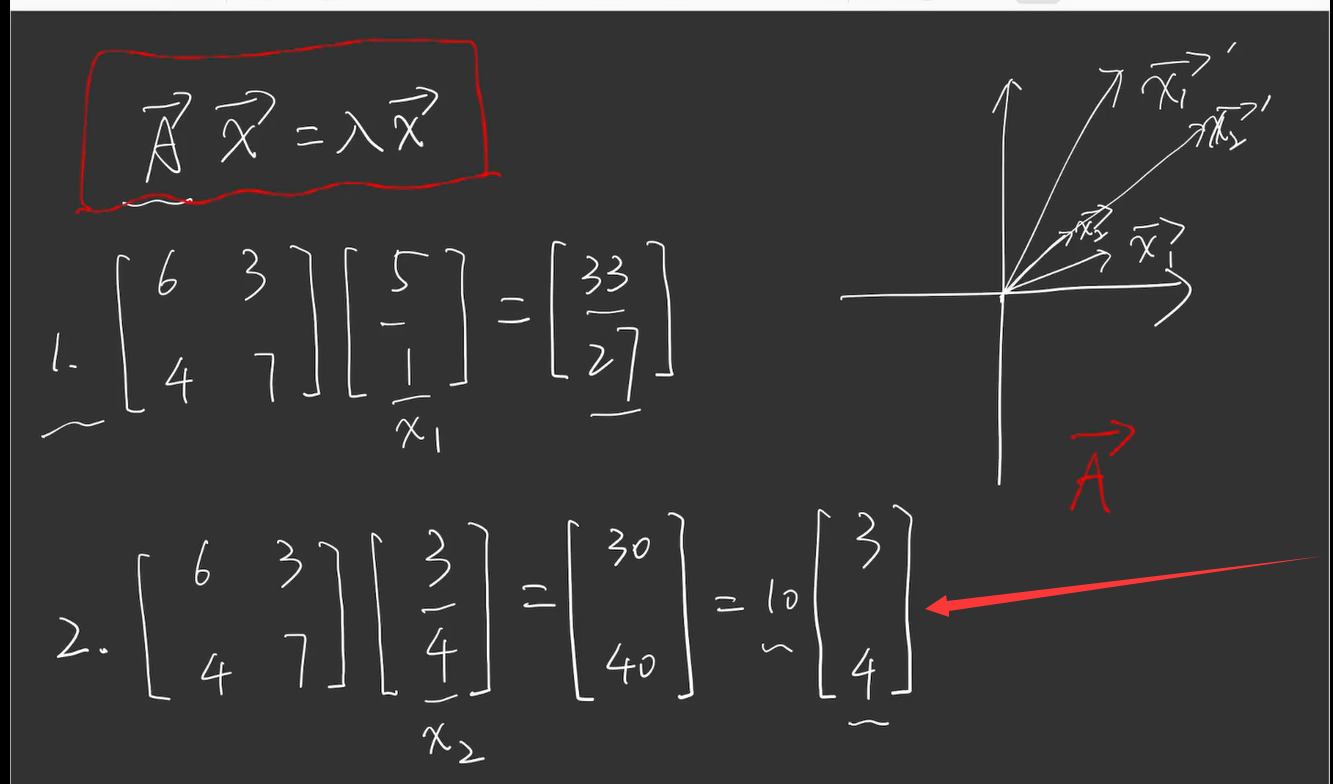
下图就是矩阵线性变换的示意图。求出矩阵的特征值为2和8,得出特征向量（1.-1）、（1.1），图形由圆形经过变换变成椭圆。

1.2 奇异值分解

• 奇异值分解常用于数据压缩和图像去噪。
  
  
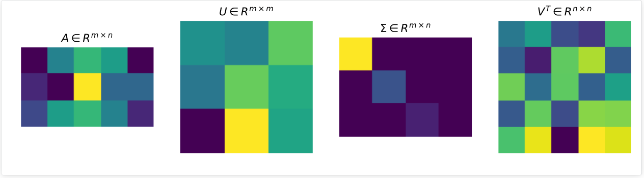
  对于奇异值分解，我们可以利用上面的图形象表示，图中方块的颜色表示值的大小，颜色越浅，值越大。对于奇异值矩阵Σ，只有其主对角线有奇异值，其余均为0。

奇异值分解在图像压缩中的应用

%matplotlib inline
import matplotlib.pyplot as plt
import matplotlib.image as mpimg
import numpy as np
 
img_eg = mpimg.imread("../img/beauty.jpg")
print(img_eg.shape
#图片的大小是600×400×3

#奇异值分解
img_temp = img_eg.reshape(600, 400 * 3)
U,Sigma,VT = np.linalg.svd(img_temp)

我们先将图片变成600×1200，再做奇异值分解。从svd函数中得到的奇异值sigma它是从大到小排列的。

# 取前60个奇异值
sval_nums = 60
img_restruct1 = (U[:,0:sval_nums]).dot(np.diag(Sigma[0:sval_nums])).dot(VT[0:sval_nums,:])
img_restruct1 = img_restruct1.reshape(600,400,3)
 
# 取前120个奇异值
sval_nums = 120
img_restruct2 = (U[:,0:sval_nums]).dot(np.diag(Sigma[0:sval_nums])).dot(VT[0:sval_nums,:])
img_restruct2 = img_restruct2.reshape(600,400,3)

#将图片显示出来看一下，对比下效果
fig, ax = plt.subplots(1,3,figsize = (24,32))
 
ax[0].imshow(img_eg)
ax[0].set(title = "src")
ax[1].imshow(img_restruct1.astype(np.uint8))
ax[1].set(title = "nums of sigma = 60")
ax[2].imshow(img_restruct2.astype(np.uint8))
ax[2].set(title = "nums of sigma = 120")

当我们取到前面120个奇异值来重构图片时，基本上已经看不出与原图片有多大的差别。如下图所示。（资料参考自网络）。

从上面的图片的压缩结果中可以看出来，奇异值可以被看作成一个矩阵的代表值，或者说，奇异值能够代表这个矩阵的信息。当奇异值越大时，它代表的信息越多。因此，我们取前面若干个最大的奇异值，就可以基本上还原出数据本身。

• 卷积神经网络-卷积层

传统的神经网络中间都是全连接层，权重矩阵的参数多，容易出现过拟合的情况。所谓过拟合，就是过度拟合了训练集上的特征，泛化能力比较差。所以采取了卷积神经网络，卷积神经网络中间包含卷积层、池化层、全连接层。卷积神经网络采用局部互联，不再是神经元和整个图片上都有连接，而是连接图片上小的局部块，也就是卷积核。参数的大小跟卷积核有关，大大的降低了参数量，使得模型更好的训练。

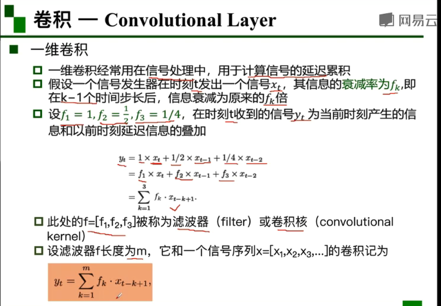
1.3 一维卷积

一维卷积经常用在信号处理中，用来计算信号的延迟累积。

1.4 二维卷积

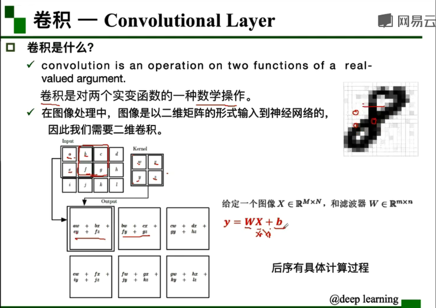
W对应于卷积核的参数，也就是权重，X对应input里的一块区域。 在卷积核进行一次卷积的时候，input里的这块区域称之为该卷积核对应的感受野（receptive field）。在经过一次卷积之后输出的结果叫做特征图。步长（stride）为1时表示卷积一次向右移动一个单位长度，当出现右边的大小不匹配时，如图：

此时在输入的两边进行补0。也就是padding的概念。

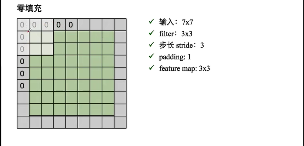
当输入为7x7x3时，此时的3可以理解为图像的3个通道，也可以理解为3个feature map。 一个3*3的filiter又包含了3个不同的权重矩阵，每一个权重矩阵对应一个通道进行运算。结果求和得到输出的feature map上的对应值。

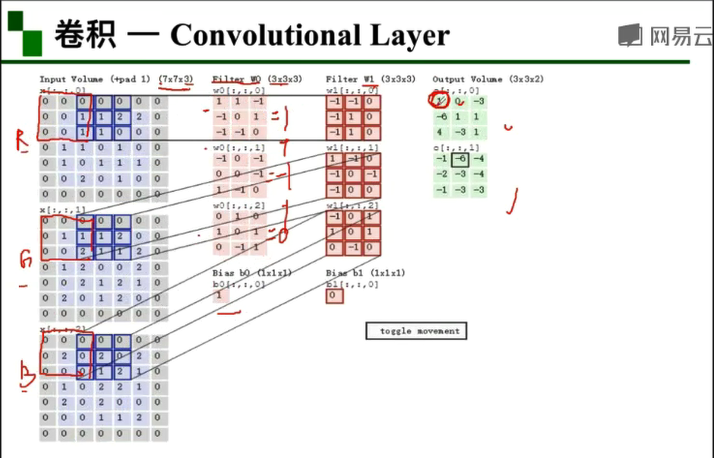
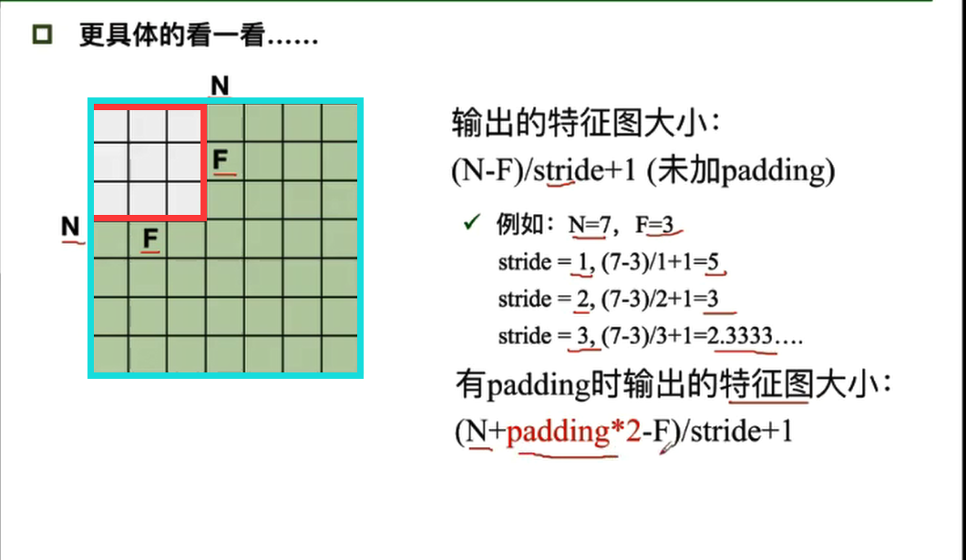
输出的特征图大小可以通过输入的大小和卷积核的大小计算得来。

深度（depth/channel）跟卷积核的个数有关，有多少个卷积核就有多少的channel。

input:32*32
filter:10,5*5    就是10个5*5的卷积核
stride:1         步长为1
padding:2        
output feature map： 输出的特征图大小就是32*32*10
（32+2*2-5）/1+1=32
参数量：(5*5+1)*10=260

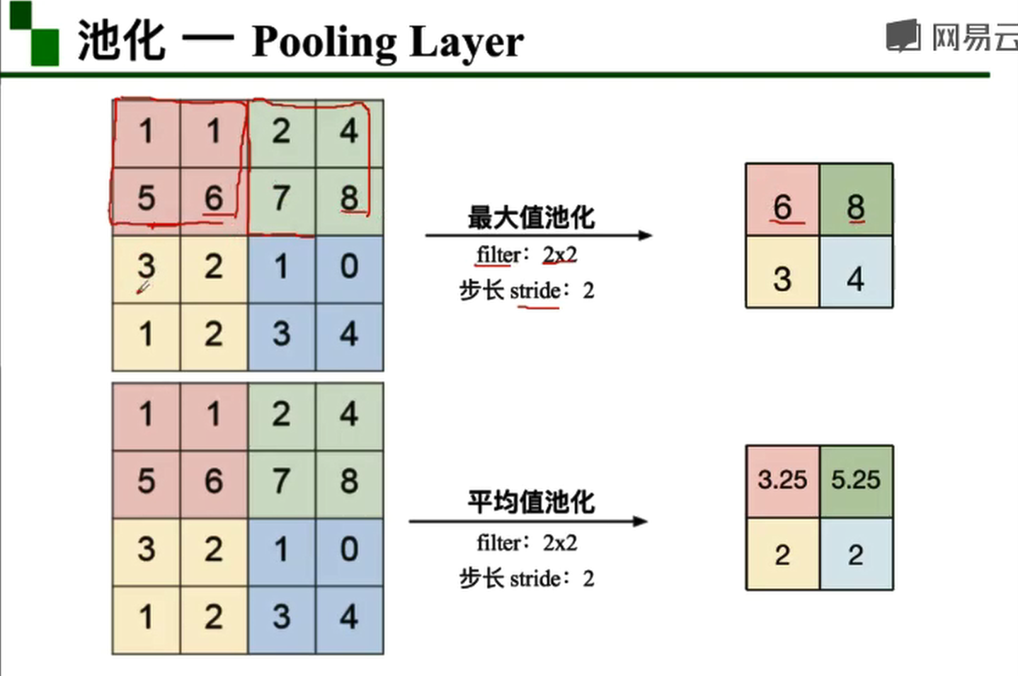
• 卷积神经网络-池化层

池化的过程更像是实现缩放的过程，在缩放的过程中保留了主要特征的同时减少参数和计算量，防止过拟合，提高模型泛化能力。池化层处于卷积层和卷积层之间 ，全连接层和全连接层之间。主要类型是最大值池化和平均值池化。池化层跟卷积层类似，也有filter和stride的概念。 常用的为最大值池化。

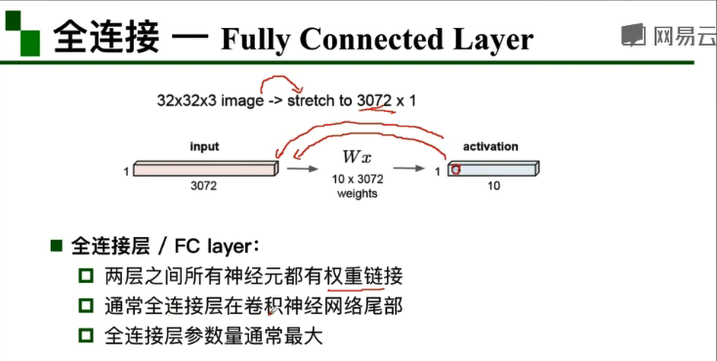
• 卷积神经网络-全连接层

全连接层通常在卷积神经网络的尾部。

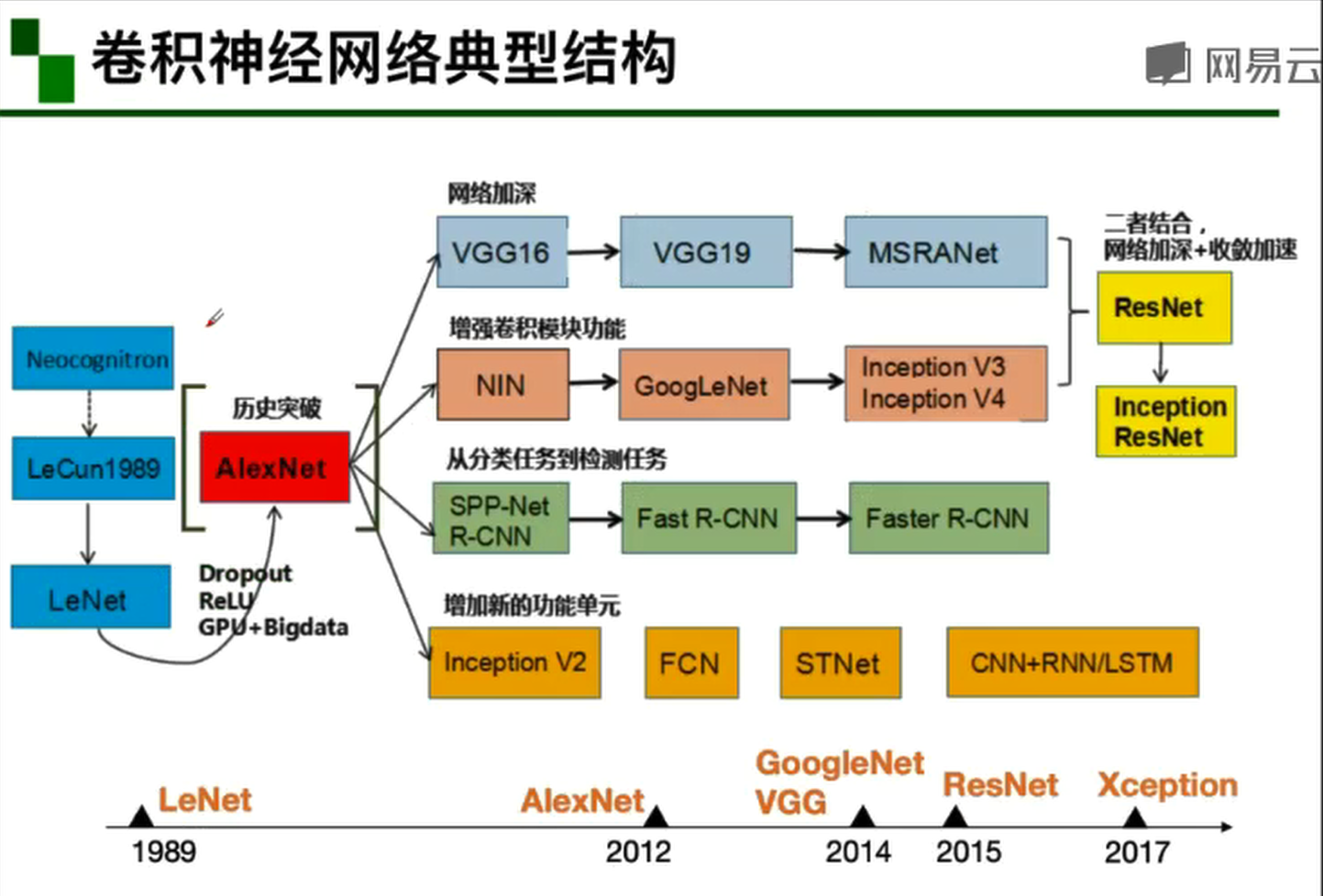
• 卷积神经网络典型结构

• 卷积神经网络典型结构-AlexNet

AlexNet是深度学习的一个转折点，之所以能够成功，原因在于：

1.大数据训练：百万级ImageNet图像数据

2.非线性激活函数：ReLu

优点：
解决了梯度消失问题（在正区间）
计算速度特别快，只需要判断输入是否大于0
收敛速度远快于sigmoid

3.防止过拟合：Dropout,Data augmentation

DropOut(随机失活)
  训练时随机关闭部分神经元，测试时整合所有神经元
Data augmentation（数据增强）
  平移、翻转、对称
  改变RGB通道强度

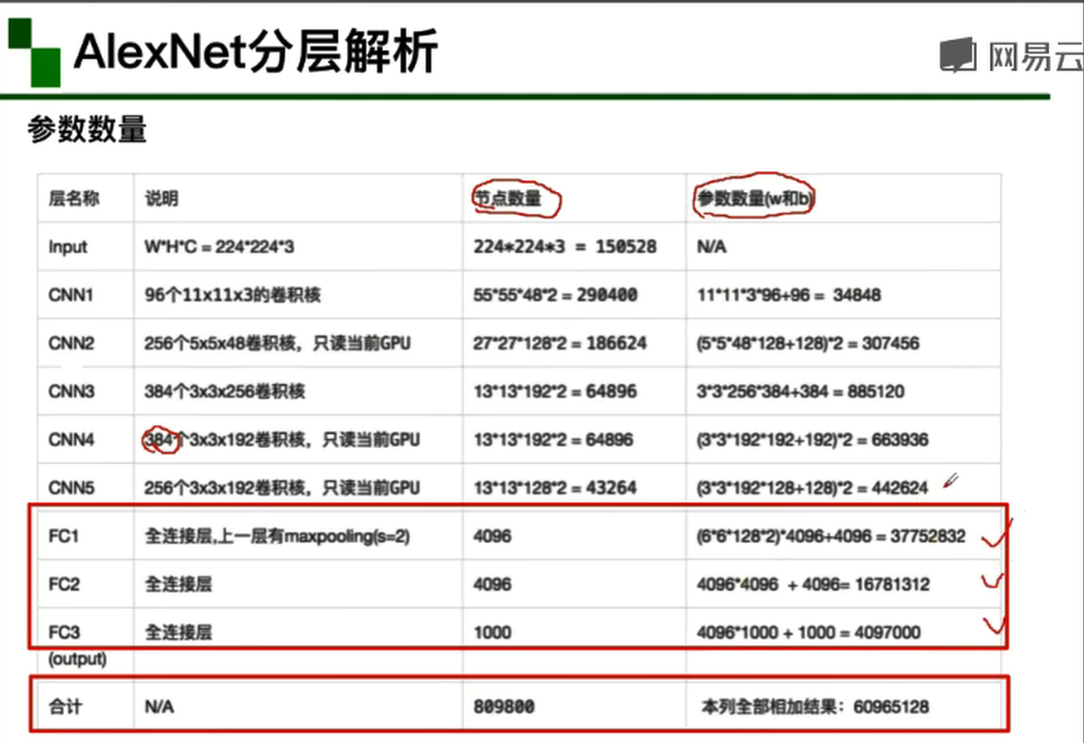
AlexNet分层解析

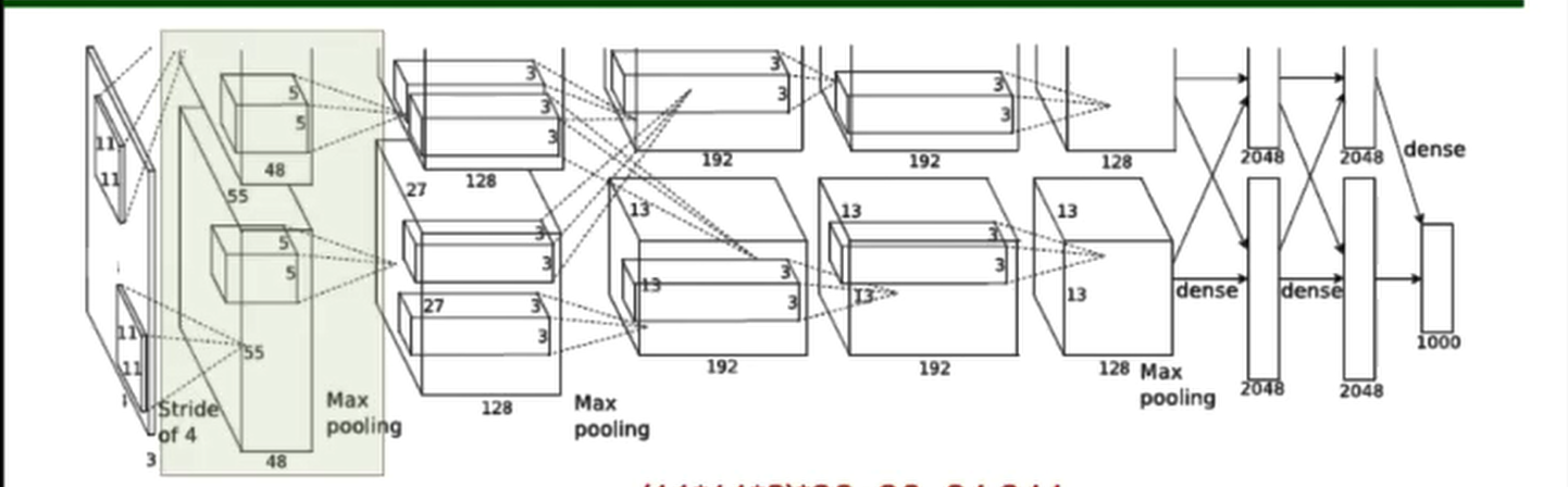
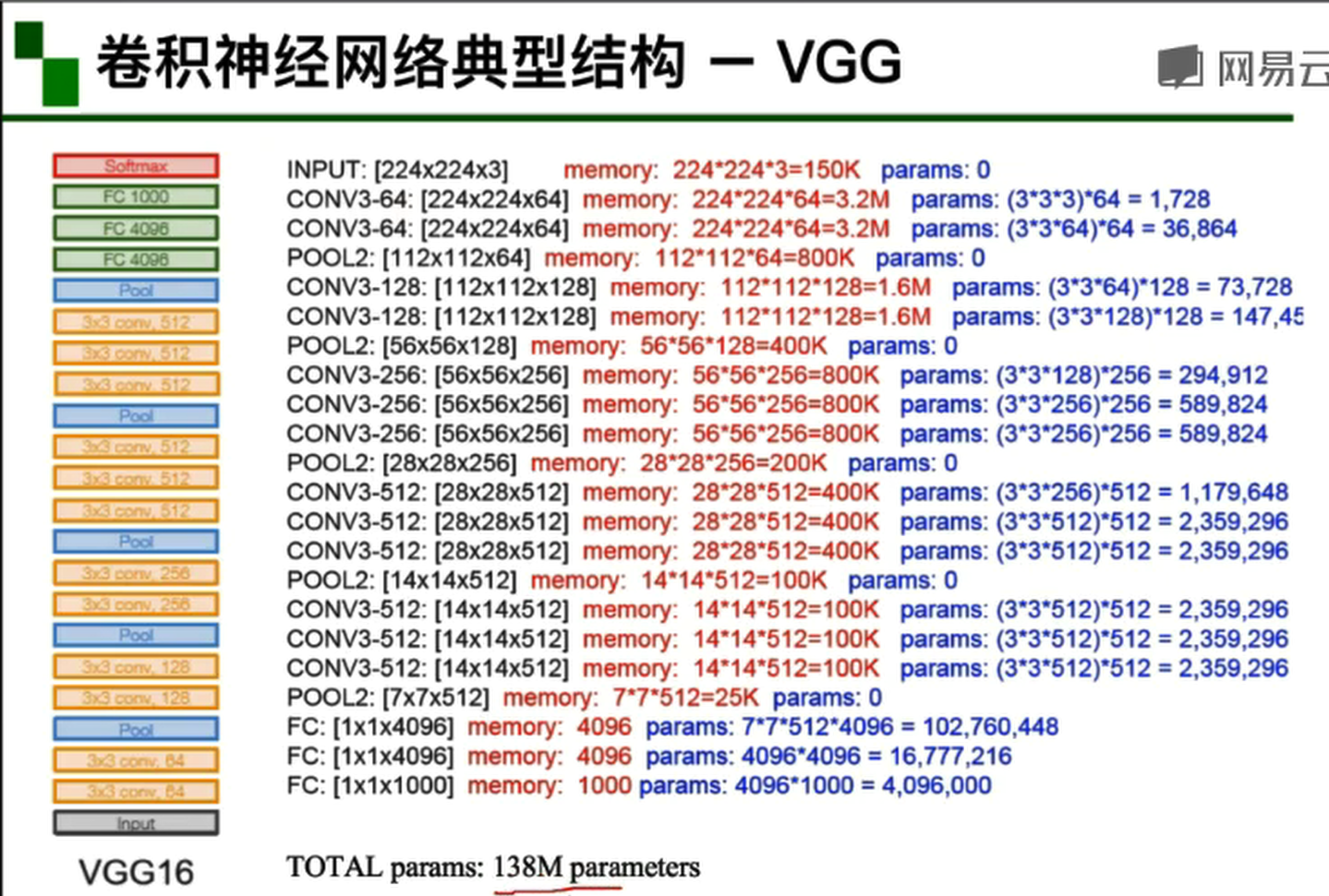
注意在池化层的参数为0。各层的feature map 的大小根据上面的公式计算即可。可以看出主要的参数位于全连接层。

 第一次卷积：卷积-ReLU-池化        224x224x3—55x55x96—27x27x96—27x27x96
 第二次卷积：卷积-ReLU-池化        27x27x96—27x27x256—13x13x256—13x13x256
 第三次卷积：卷积-ReLU                  13x13x256—13x13x384—13x13x384
 第四次卷积：卷积-ReLU                  13x13x384—13x13x384—13x13x384
 第五次卷积：卷积-ReLU-池化         13x13x384—13x13x256—13x13x256—6x6x256
 第六次卷积：全连接-ReLU-DropOut      6x6x256—4096—4096—4096
 第七次卷积：全连接-ReLU-DropOut      4096—4096—4096—4096
 第八次卷积：全连接-SoftMax                  4096—1000

• 卷积神经网络典型结构-ZFNet

网络结构与AlexNet相同
将卷积层1中的感受野大小由11*11改为7*7
卷积层3,4,5中的滤波器个数由384,384,256改为512，512,1024

• 卷积神经网络典型结构-VGG

VGG是一个更深的网络，将AlexNet的深度由8层加深到16和19层。

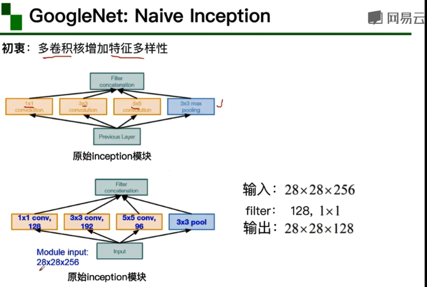
• 卷积神经网络典型结构-GoogleNet

GoogleNet不像VGG只在深度上做了加深，而是在结构上发生了改进，加入了多个inception模块和一个分类结构，包括两个辅助分类器（防止模型较深时出现的梯度消失问题），作用不是很大，所以在inception V3里去掉了辅助分类器。

网络总体结构：
   网络包含22个带参数的层，（如果考虑池化层就是27层），独立成块的层数约有100个
   参数量是AlexNet的1/12
   除了分类的全连接层之外没有其他的全连接层

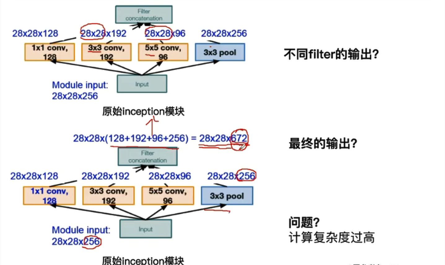
对channel上进行一个串联，就是28x28x(128+192+96+256)=28x28x678,经过max pooling之后672并不会改变，随着模型不断地加深，channel不断增大，计算量就会变得复杂。

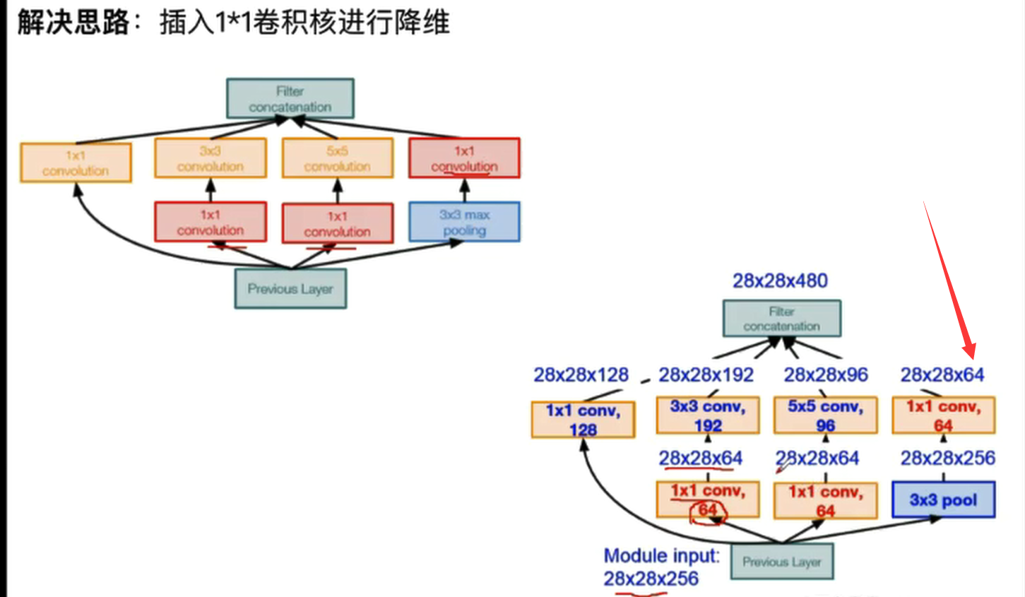
在inceptionV2中通过插入1*1的卷积核进行降维。在max pooling之后加上一个卷积核，从而可以改变深度，减少参数量。

inceptionV3对V2的参数量进一步降低，对V2的5x5的卷积核变成两个3x3的卷积核。 两种情况得到的输出是一样的，且5x5的参数量=（5x5）+1=26,3x3的参数量=(（3x3）+1)=20。从而降低了参数量。第二增加了非线性激活函数，使网络产生更多独立特征，表征能力更强。

Stem部分跟AlexNet很像，中间采用一些inception结构堆叠。最后一个全连接层输出类别数目。

• 卷积神经网络典型结构-ResNet

残差学习网络，深度有152层。

\[传统结构：f(g(h(x)))’=f‘g'h' 残差block：(f(g(h(x)+x)+x)+x)’=(f’+1)(g'+1)(h'+1) \]

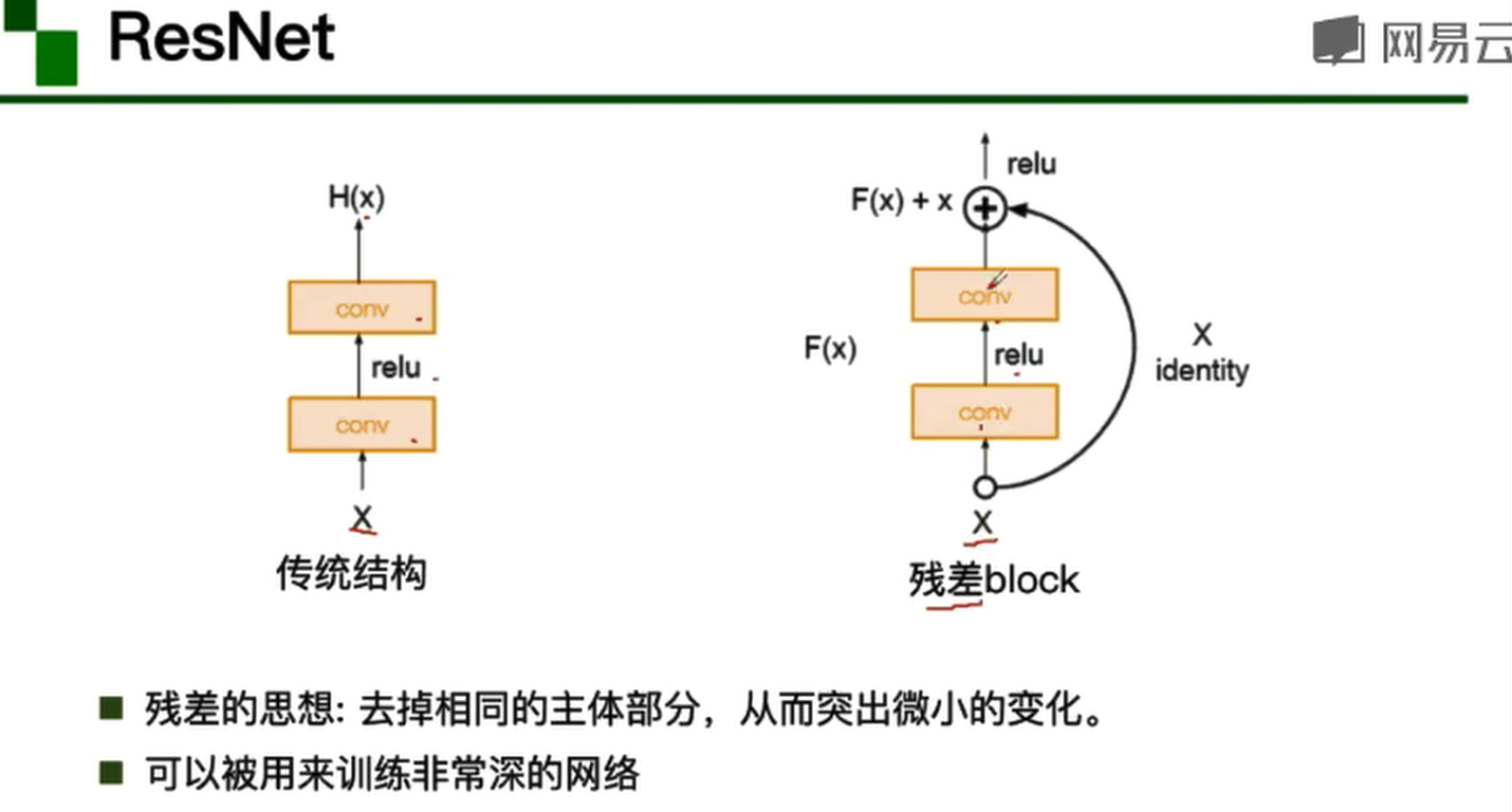
可以看出传统结构的导数可能出现的等于0 的情况，也就是会出现梯度消失的问题，而残差结构不会出现等于0的情况。

二、代码练习

2.1 MNIST数据集分类

2.1.1 加载数据

input_size  = 28*28   # MNIST上的图像尺寸是 28x28
output_size = 10      # 类别为 0 到 9 的数字，因此为十类

train_loader = torch.utils.data.DataLoader(
    datasets.MNIST('./data', train=True, download=True,
        transform=transforms.Compose(
            [transforms.ToTensor(),
             transforms.Normalize((0.1307,), (0.3081,))])),
    batch_size=64, shuffle=True)

test_loader = torch.utils.data.DataLoader(
    datasets.MNIST('./data', train=False, transform=transforms.Compose([
             transforms.ToTensor(),
             transforms.Normalize((0.1307,), (0.3081,))])),
    batch_size=1000, shuffle=True)

PyTorch里包含了 MNIST， CIFAR10 等常用数据集，调用 torchvision.datasets 即可把这些数据由远程下载到本地，下面给出MNIST的使用方法： torchvision.datasets.MNIST(root, train=True, transform=None, target_transform=None, download=False) root 为数据集下载到本地后的根目录，包括 training.pt 和 test.pt 文件 train，如果设置为True，从training.pt创建数据集，否则从test.pt创建。 download，如果设置为True, 从互联网下载数据并放到root文件夹下 transform, 一种函数或变换，输入PIL图片，返回变换之后的数据。 target_transform 一种函数或变换，输入目标，进行变换。 另外值得注意的是，DataLoader是一个比较重要的类，提供的常用操作有：batch_size(每个batch的大小), shuffle(是否进行随机打乱顺序的操作), num_workers(加载数据的时候使用几个子进程)。

2.1.2显示数据集中的部分图像

plt.figure(figsize=(8, 5))
for i in range(20):
    plt.subplot(4, 5, i + 1)
    image, _ = train_loader.dataset.__getitem__(i)
    plt.imshow(image.squeeze().numpy(),'gray')
    plt.axis('off');

2.1.3创建网络

class FC2Layer(nn.Module):
    def __init__(self, input_size, n_hidden, output_size):
        # nn.Module子类的函数必须在构造函数中执行父类的构造函数
        # 下式等价于nn.Module.__init__(self)        
        super(FC2Layer, self).__init__()
        self.input_size = input_size
        # 这里直接用 Sequential 就定义了网络，注意要和下面 CNN 的代码区分开
        self.network = nn.Sequential(
            nn.Linear(input_size, n_hidden), 
            nn.ReLU(), 
            nn.Linear(n_hidden, n_hidden), 
            nn.ReLU(), 
            nn.Linear(n_hidden, output_size), 
            nn.LogSoftmax(dim=1)
        )
    def forward(self, x):
        # view一般出现在model类的forward函数中，用于改变输入或输出的形状
        # x.view(-1, self.input_size) 的意思是多维的数据展成二维
        # 代码指定二维数据的列数为 input_size=784，行数 -1 表示我们不想算，电脑会自己计算对应的数字
        # 在 DataLoader 部分，我们可以看到 batch_size 是64，所以得到 x 的行数是64
        # 大家可以加一行代码：print(x.cpu().numpy().shape)
        # 训练过程中，就会看到 (64, 784) 的输出，和我们的预期是一致的

        # forward 函数的作用是，指定网络的运行过程，这个全连接网络可能看不啥意义，
        # 下面的CNN网络可以看出 forward 的作用。
        x = x.view(-1, self.input_size)
        return self.network(x)
    


class CNN(nn.Module):
    def __init__(self, input_size, n_feature, output_size):
        # 执行父类的构造函数，所有的网络都要这么写
        super(CNN, self).__init__()
        # 下面是网络里典型结构的一些定义，一般就是卷积和全连接
        # 池化、ReLU一类的不用在这里定义
        self.n_feature = n_feature
        self.conv1 = nn.Conv2d(in_channels=1, out_channels=n_feature, kernel_size=5)
        self.conv2 = nn.Conv2d(n_feature, n_feature, kernel_size=5)
        self.fc1 = nn.Linear(n_feature*4*4, 50)
        self.fc2 = nn.Linear(50, 10)    
    
    # 下面的 forward 函数，定义了网络的结构，按照一定顺序，把上面构建的一些结构组织起来
    # 意思就是，conv1, conv2 等等的，可以多次重用
    def forward(self, x, verbose=False):
        x = self.conv1(x)
        x = F.relu(x)
        x = F.max_pool2d(x, kernel_size=2)
        x = self.conv2(x)
        x = F.relu(x)
        x = F.max_pool2d(x, kernel_size=2)
        x = x.view(-1, self.n_feature*4*4)
        x = self.fc1(x)
        x = F.relu(x)
        x = self.fc2(x)
        x = F.log_softmax(x, dim=1)
        return x

2.1.4定义训练和测试函数

# 训练函数
def train(model):
    model.train()
    # 主里从train_loader里，64个样本一个batch为单位提取样本进行训练
    for batch_idx, (data, target) in enumerate(train_loader):
        # 把数据送到GPU中
        data, target = data.to(device), target.to(device)

        optimizer.zero_grad()
        output = model(data)
        loss = F.nll_loss(output, target)
        loss.backward()
        optimizer.step()
        if batch_idx % 100 == 0:
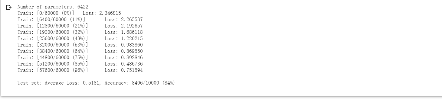
            print('Train: [{}/{} ({:.0f}%)]\tLoss: {:.6f}'.format(
                batch_idx * len(data), len(train_loader.dataset),
                100. * batch_idx / len(train_loader), loss.item()))


def test(model):
    model.eval()
    test_loss = 0
    correct = 0
    for data, target in test_loader:
        # 把数据送到GPU中
        data, target = data.to(device), target.to(device)
        # 把数据送入模型，得到预测结果
        output = model(data)
        # 计算本次batch的损失，并加到 test_loss 中
        test_loss += F.nll_loss(output, target, reduction='sum').item()
        # get the index of the max log-probability，最后一层输出10个数，
        # 值最大的那个即对应着分类结果，然后把分类结果保存在 pred 里
        pred = output.data.max(1, keepdim=True)[1]
        # 将 pred 与 target 相比，得到正确预测结果的数量，并加到 correct 中
        # 这里需要注意一下 view_as ，意思是把 target 变成维度和 pred 一样的意思                                                
        correct += pred.eq(target.data.view_as(pred)).cpu().sum().item()

    test_loss /= len(test_loader.dataset)
    accuracy = 100. * correct / len(test_loader.dataset)
    print('\nTest set: Average loss: {:.4f}, Accuracy: {}/{} ({:.0f}%)\n'.format(
        test_loss, correct, len(test_loader.dataset),
        accuracy))

2.1.5在小型全连接网络上训练（Fully-connected network）

n_hidden = 8 # number of hidden units

model_fnn = FC2Layer(input_size, n_hidden, output_size)
model_fnn.to(device)
optimizer = optim.SGD(model_fnn.parameters(), lr=0.01, momentum=0.5)
print('Number of parameters: {}'.format(get_n_params(model_fnn)))

train(model_fnn)
test(model_fnn)

2.1.6在卷积神经网络上训练与测试：

# Training settings 
n_features = 6 # number of feature maps

model_cnn = CNN(input_size, n_features, output_size)
model_cnn.to(device)
optimizer = optim.SGD(model_cnn.parameters(), lr=0.01, momentum=0.5)
print('Number of parameters: {}'.format(get_n_params(model_cnn)))

train(model_cnn)
test(model_cnn)

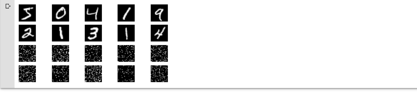
2.1.7打乱像素顺序再次在两个网络上训练与测试

# 这里解释一下 torch.randperm 函数，给定参数n，返回一个从0到n-1的随机整数排列
perm = torch.randperm(784)
plt.figure(figsize=(8, 4))
for i in range(10):
    image, _ = train_loader.dataset.__getitem__(i)
    # permute pixels
    image_perm = image.view(-1, 28*28).clone()
    image_perm = image_perm[:, perm]
    image_perm = image_perm.view(-1, 1, 28, 28)
    plt.subplot(4, 5, i + 1)
    plt.imshow(image.squeeze().numpy(), 'gray')
    plt.axis('off')
    plt.subplot(4, 5, i + 11)
    plt.imshow(image_perm.squeeze().numpy(), 'gray')
    plt.axis('off')

# 对每个 batch 里的数据，打乱像素顺序的函数
def perm_pixel(data, perm):
    # 转化为二维矩阵
    data_new = data.view(-1, 28*28)
    # 打乱像素顺序
    data_new = data_new[:, perm]
    # 恢复为原来4维的 tensor
    data_new = data_new.view(-1, 1, 28, 28)
    return data_new

# 训练函数
def train_perm(model, perm):
    model.train()
    for batch_idx, (data, target) in enumerate(train_loader):
        data, target = data.to(device), target.to(device)
        # 像素打乱顺序
        data = perm_pixel(data, perm)

        optimizer.zero_grad()
        output = model(data)
        loss = F.nll_loss(output, target)
        loss.backward()
        optimizer.step()
        if batch_idx % 100 == 0:
            print('Train: [{}/{} ({:.0f}%)]\tLoss: {:.6f}'.format(
                batch_idx * len(data), len(train_loader.dataset),
                100. * batch_idx / len(train_loader), loss.item()))

# 测试函数
def test_perm(model, perm):
    model.eval()
    test_loss = 0
    correct = 0
    for data, target in test_loader:
        data, target = data.to(device), target.to(device)

        # 像素打乱顺序
        data = perm_pixel(data, perm)

        output = model(data)
        test_loss += F.nll_loss(output, target, reduction='sum').item()
        pred = output.data.max(1, keepdim=True)[1]                                            
        correct += pred.eq(target.data.view_as(pred)).cpu().sum().item()

    test_loss /= len(test_loader.dataset)
    accuracy = 100. * correct / len(test_loader.dataset)
    print('\nTest set: Average loss: {:.4f}, Accuracy: {}/{} ({:.0f}%)\n'.format(
        test_loss, correct, len(test_loader.dataset),
        accuracy))

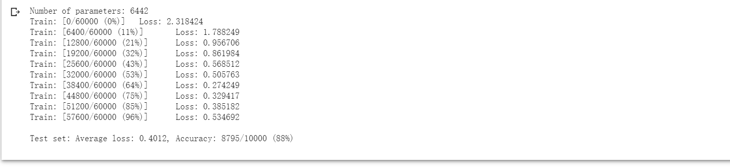
2.1.8在全连接网络上训练与测试

perm = torch.randperm(784)
n_hidden = 8 # number of hidden units

model_fnn = FC2Layer(input_size, n_hidden, output_size)
model_fnn.to(device)
optimizer = optim.SGD(model_fnn.parameters(), lr=0.01, momentum=0.5)
print('Number of parameters: {}'.format(get_n_params(model_fnn)))

train_perm(model_fnn, perm)
test_perm(model_fnn, perm)

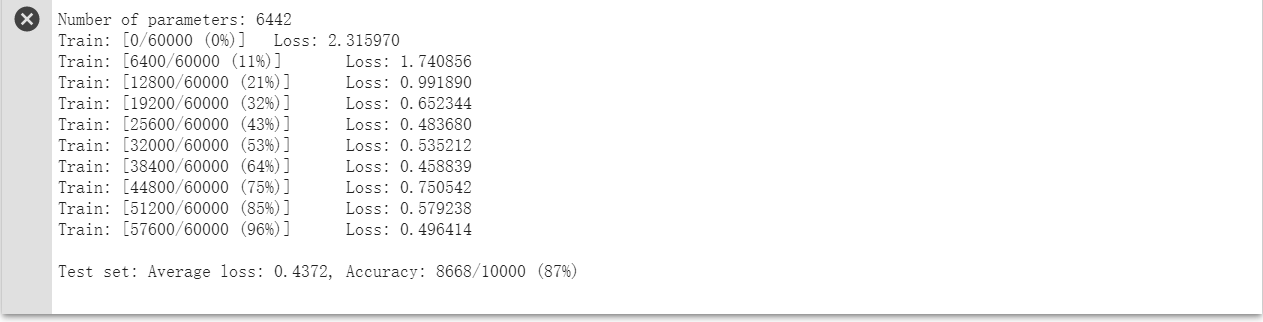
2.1.9在卷积神经网络上训练与测试：

perm = torch.randperm(784)
n_features = 6 # number of feature maps

model_cnn = CNN(input_size, n_features, output_size)
model_cnn.to(device)
optimizer = optim.SGD(model_cnn.parameters(), lr=0.01, momentum=0.5)
print('Number of parameters: {}'.format(get_n_params(model_cnn)))

train_perm(model_cnn, perm)
test_perm(model_cnn, perm)

2.2 CIFAR10 数据集分类

2.2.1定义网络、损失函数和优化器

class Net(nn.Module):
    def __init__(self):
        super(Net, self).__init__()
        self.conv1 = nn.Conv2d(3, 6, 5)
        self.pool = nn.MaxPool2d(2, 2)
        self.conv2 = nn.Conv2d(6, 16, 5)
        self.fc1 = nn.Linear(16 * 5 * 5, 120)
        self.fc2 = nn.Linear(120, 84)
        self.fc3 = nn.Linear(84, 10)

    def forward(self, x):
        x = self.pool(F.relu(self.conv1(x)))
        x = self.pool(F.relu(self.conv2(x)))
        x = x.view(-1, 16 * 5 * 5)
        x = F.relu(self.fc1(x))
        x = F.relu(self.fc2(x))
        x = self.fc3(x)
        return x

# 网络放到GPU上
net = Net().to(device)
criterion = nn.CrossEntropyLoss()
optimizer = optim.Adam(net.parameters(), lr=0.001)

2.2.2训练网络

for epoch in range(10):  # 重复多轮训练
    for i, (inputs, labels) in enumerate(trainloader):
        inputs = inputs.to(device)
        labels = labels.to(device)
        # 优化器梯度归零
        optimizer.zero_grad()
        # 正向传播 +　反向传播 + 优化 
        outputs = net(inputs)
        loss = criterion(outputs, labels)
        loss.backward()
        optimizer.step()
        # 输出统计信息
        if i % 100 == 0:   
            print('Epoch: %d Minibatch: %5d loss: %.3f' %(epoch + 1, i + 1, loss.item()))

print('Finished Training')

2.2.3网络在数据集上的表现

correct = 0
total = 0

for data in testloader:
    images, labels = data
    images, labels = images.to(device), labels.to(device)
    outputs = net(images)
    _, predicted = torch.max(outputs.data, 1)
    total += labels.size(0)
    correct += (predicted == labels).sum().item()

print('Accuracy of the network on the 10000 test images: %d %%' % (
    100 * correct / total))

Epoch: 1 Minibatch:     1 loss: 2.300
Epoch: 1 Minibatch:   101 loss: 1.944
Epoch: 1 Minibatch:   201 loss: 1.765
Epoch: 1 Minibatch:   301 loss: 1.846
Epoch: 1 Minibatch:   401 loss: 1.577
Epoch: 1 Minibatch:   501 loss: 1.566
Epoch: 1 Minibatch:   601 loss: 1.663
Epoch: 1 Minibatch:   701 loss: 1.921
Epoch: 2 Minibatch:     1 loss: 1.692
Epoch: 2 Minibatch:   101 loss: 1.282
Epoch: 2 Minibatch:   201 loss: 1.298
Epoch: 2 Minibatch:   301 loss: 1.272
Epoch: 2 Minibatch:   401 loss: 1.149
Epoch: 2 Minibatch:   501 loss: 1.290
Epoch: 2 Minibatch:   601 loss: 1.286
Epoch: 2 Minibatch:   701 loss: 1.142
Epoch: 3 Minibatch:     1 loss: 1.333
Epoch: 3 Minibatch:   101 loss: 1.329
Epoch: 3 Minibatch:   201 loss: 1.155
Epoch: 3 Minibatch:   301 loss: 1.485
Epoch: 3 Minibatch:   401 loss: 1.067
Epoch: 3 Minibatch:   501 loss: 1.128
Epoch: 3 Minibatch:   601 loss: 1.042
Epoch: 3 Minibatch:   701 loss: 1.071
Epoch: 4 Minibatch:     1 loss: 0.965
Epoch: 4 Minibatch:   101 loss: 1.206
Epoch: 4 Minibatch:   201 loss: 0.803
Epoch: 4 Minibatch:   301 loss: 0.957
Epoch: 4 Minibatch:   401 loss: 1.367
Epoch: 4 Minibatch:   501 loss: 1.183
Epoch: 4 Minibatch:   601 loss: 1.283
Epoch: 4 Minibatch:   701 loss: 1.266
Epoch: 5 Minibatch:     1 loss: 0.926
Epoch: 5 Minibatch:   101 loss: 1.308
Epoch: 5 Minibatch:   201 loss: 0.964
Epoch: 5 Minibatch:   301 loss: 1.091
Epoch: 5 Minibatch:   401 loss: 1.195
Epoch: 5 Minibatch:   501 loss: 1.081
Epoch: 5 Minibatch:   601 loss: 1.012
Epoch: 5 Minibatch:   701 loss: 1.215
Epoch: 6 Minibatch:     1 loss: 0.951
Epoch: 6 Minibatch:   101 loss: 1.154
Epoch: 6 Minibatch:   201 loss: 0.968
Epoch: 6 Minibatch:   301 loss: 1.096
Epoch: 6 Minibatch:   401 loss: 1.046
Epoch: 6 Minibatch:   501 loss: 0.985
Epoch: 6 Minibatch:   601 loss: 0.750
Epoch: 6 Minibatch:   701 loss: 0.901
Epoch: 7 Minibatch:     1 loss: 1.086
Epoch: 7 Minibatch:   101 loss: 1.038
Epoch: 7 Minibatch:   201 loss: 0.978
Epoch: 7 Minibatch:   301 loss: 1.006
Epoch: 7 Minibatch:   401 loss: 0.811
Epoch: 7 Minibatch:   501 loss: 0.958
Epoch: 7 Minibatch:   601 loss: 0.753
Epoch: 7 Minibatch:   701 loss: 0.985
Epoch: 8 Minibatch:     1 loss: 1.070
Epoch: 8 Minibatch:   101 loss: 0.981
Epoch: 8 Minibatch:   201 loss: 0.748
Epoch: 8 Minibatch:   301 loss: 0.844
Epoch: 8 Minibatch:   401 loss: 0.785
Epoch: 8 Minibatch:   501 loss: 0.887
Epoch: 8 Minibatch:   601 loss: 0.617
Epoch: 8 Minibatch:   701 loss: 0.939
Epoch: 9 Minibatch:     1 loss: 0.778
Epoch: 9 Minibatch:   101 loss: 0.586
Epoch: 9 Minibatch:   201 loss: 0.957
Epoch: 9 Minibatch:   301 loss: 1.123
Epoch: 9 Minibatch:   401 loss: 1.104
Epoch: 9 Minibatch:   501 loss: 0.842
Epoch: 9 Minibatch:   601 loss: 0.812
Epoch: 9 Minibatch:   701 loss: 0.825
Epoch: 10 Minibatch:     1 loss: 0.716
Epoch: 10 Minibatch:   101 loss: 0.833
Epoch: 10 Minibatch:   201 loss: 0.977
Epoch: 10 Minibatch:   301 loss: 0.910
Epoch: 10 Minibatch:   401 loss: 1.036
Epoch: 10 Minibatch:   501 loss: 0.896
Epoch: 10 Minibatch:   601 loss: 0.834
Epoch: 10 Minibatch:   701 loss: 0.872
Finished Training

2.2.4网络在整个数据集上的表现：

correct = 0
total = 0

for data in testloader:
    images, labels = data
    images, labels = images.to(device), labels.to(device)
    outputs = net(images)
    _, predicted = torch.max(outputs.data, 1)
    total += labels.size(0)
    correct += (predicted == labels).sum().item()

print('Accuracy of the network on the 10000 test images: %d %%' % (
    100 * correct / total))

2.3使用 VGG16 对 CIFAR10 分类

2.3.1建立VGG16模型

class VGG(nn.Module):
    def __init__(self):
        super(VGG, self).__init__()
        self.cfg = [64, 'M', 128, 'M', 256, 256, 'M', 512, 512, 'M', 512, 512, 'M']
        self.features = self._make_layers(cfg)
        self.classifier = nn.Linear(2048, 10)

    def forward(self, x):
        out = self.features(x)
        out = out.view(out.size(0), -1)
        out = self.classifier(out)
        return out

    def _make_layers(self, cfg):
        layers = []
        in_channels = 3
        for x in cfg:
            if x == 'M':
                layers += [nn.MaxPool2d(kernel_size=2, stride=2)]
            else:
                layers += [nn.Conv2d(in_channels, x, kernel_size=3, padding=1),
                           nn.BatchNorm2d(x),
                           nn.ReLU(inplace=True)]
                in_channels = x
        layers += [nn.AvgPool2d(kernel_size=1, stride=1)]
        return nn.Sequential(*layers)
# 网络放到GPU上
net = VGG().to(device)
criterion = nn.CrossEntropyLoss()
optimizer = optim.Adam(net.parameters(), lr=0.001)

2.3.2对数据集分类

correct = 0
total = 0

for data in testloader:
    images, labels = data
    images, labels = images.to(device), labels.to(device)
    outputs = net(images)
    _, predicted = torch.max(outputs.data, 1)
    total += labels.size(0)
    correct += (predicted == labels).sum().item()

print('Accuracy of the network on the 10000 test images: %.2f %%' % (
    100 * correct / total))

Accuracy of the network on the 10000 test images: 84.48 %

2.4使用VGG模型迁移学习进行猫狗大战

import numpy as np
import matplotlib.pyplot as plt
import os
import torch
import torch.nn as nn
import torchvision
from torchvision import models,transforms,datasets
import time
import json


# 判断是否存在GPU设备
device = torch.device("cuda:0" if torch.cuda.is_available() else "cpu")
print('Using gpu: %s ' % torch.cuda.is_available())

Using gpu: True 

2.4.1下载数据

! wget https://static.leiphone.com/cat_dog.rar

pip install rarfile

Collecting rarfile
  Downloading https://files.pythonhosted.org/packages/95/f4/c92fab227c7457e3b76a4096ccb655ded9deac869849cb03afbe55dfdc1e/rarfile-4.0-py3-none-any.whl
Installing collected packages: rarfile
Successfully installed rarfile-4.0

2.4.2解压文件

import rarfile
path = "cat_dog.rar"
path2 = "/content/"
rf = rarfile.RarFile(path) 
rf.extractall(path2)

normalize = transforms.Normalize(mean=[0.485, 0.456, 0.406], std=[0.229, 0.224, 0.225])

vgg_format_train = transforms.Compose([
                transforms.RandomRotation(30),# 随机旋转
                transforms.CenterCrop(224),
                transforms.ToTensor(),
                normalize,
                
            ])

vgg_format = transforms.Compose([
                transforms.CenterCrop(224),
                transforms.ToTensor(),
                normalize,
            ])

data_dir = './cat_dog/'

# 利用ImageFolder进行分类文件夹加载
# 两种加载数据集的方法
dsets = {x: datasets.ImageFolder(os.path.join(data_dir, x), vgg_format)
         for x in ['train', 'val']}

tsets = {y: datasets.ImageFolder(os.path.join(data_dir, y), vgg_format)
        for y in ['test']}
dset_classes = dsets['train'].classes
dset_sizes = {x: len(dsets[x]) for x in ['train', 'val']}

# 通过下面代码可以查看 dsets 的一些属性

print(dsets['train'].classes)
print(dsets['train'].class_to_idx)
print(dsets['train'].imgs[:5])
print('dset_sizes: ', dset_sizes)

['Cat', 'Dog']
{'Cat': 0, 'Dog': 1}
[('./cat_dog/train/Cat/cat_0.jpg', 0), ('./cat_dog/train/Cat/cat_1.jpg', 0), ('./cat_dog/train/Cat/cat_10.jpg', 0), ('./cat_dog/train/Cat/cat_100.jpg', 0), ('./cat_dog/train/Cat/cat_1000.jpg', 0)]
dset_sizes:  {'train': 20000, 'val': 2000}

oader_train = torch.utils.data.DataLoader(dsets['train'], batch_size=64, shuffle=True, num_workers=6)
loader_valid = torch.utils.data.DataLoader(dsets['val'], batch_size=5, shuffle=False, num_workers=6)
loader_test = torch.utils.data.DataLoader(tsets['test'],batch_size=5,shuffle=False,num_workers=6)
'''
valid 数据一共有2000张图，每个batch是5张，因此，下面进行遍历一共会输出到 400
同时，把第一个 batch 保存到 inputs_try, labels_try，分别查看
'''
count = 1
for data in loader_valid:
    #print(count, end='\n')
    if count == 1:
        inputs_try,labels_try = data
    count +=1

print(labels_try)
print(inputs_try.shape)

tensor([0, 0, 0, 0, 0])
torch.Size([5, 3, 224, 224])

# 显示图片的小程序

def imshow(inp, title=None):
#   Imshow for Tensor.
    inp = inp.numpy().transpose((1, 2, 0))
    mean = np.array([0.485, 0.456, 0.406])
    std = np.array([0.229, 0.224, 0.225])
    inp = np.clip(std * inp + mean, 0,1)
    plt.imshow(inp)
    if title is not None:
        plt.title(title)
    plt.pause(0.001)  # pause a bit so that plots are updated
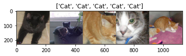
# 显示 labels_try 的5张图片，即valid里第一个batch的5张图片
out = torchvision.utils.make_grid(inputs_try)
imshow(out, title=[dset_classes[x] for x in labels_try])

2.4.3创建VGG Model

!wget https://s3.amazonaws.com/deep-learning-models/image-models/imagenet_class_index.json

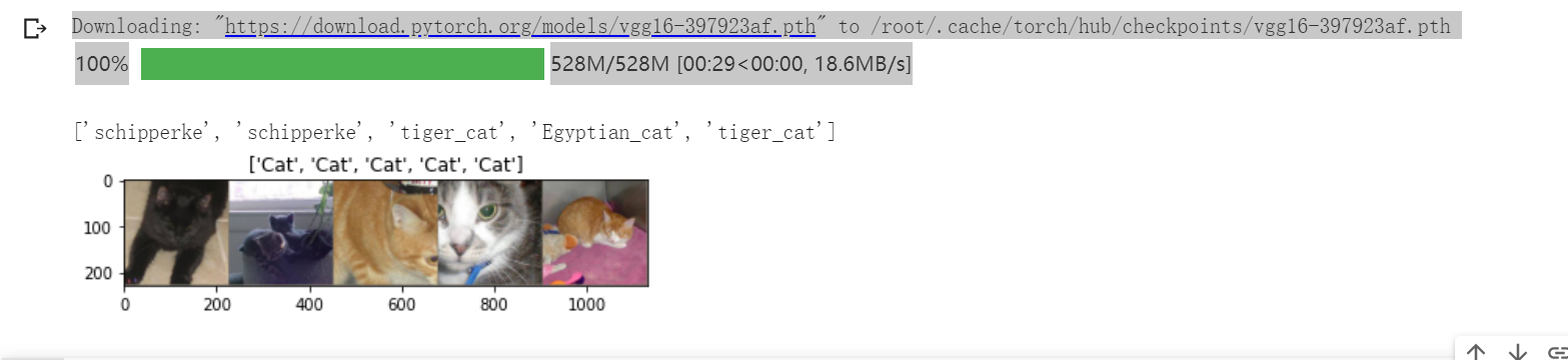
model_vgg = models.vgg16(pretrained=True)

with open('./imagenet_class_index.json') as f:
    class_dict = json.load(f)
dic_imagenet = [class_dict[str(i)][1] for i in range(len(class_dict))]

inputs_try , labels_try = inputs_try.to(device), labels_try.to(device)
model_vgg = model_vgg.to(device)

outputs_try = model_vgg(inputs_try)

#print(outputs_try)
#print(outputs_try.shape)
#tensor([[-4.6803, -3.0721, -4.2074,  ..., -8.1783, -1.4379,  5.2827],
#        [-2.4916, -3.3212,  1.3284,  ..., -4.5295, -0.9055,  4.1661],
#        [-1.4204, -0.0192, -2.6073,  ..., -0.2028,  3.1158,  3.8306],
#        [-4.0369, -2.0386, -2.7258,  ..., -5.3328,  4.3880,  1.6959],
#        [-1.8230,  4.3508, -3.3690,  ..., -2.3910,  3.7018,  5.3185]],
#       device='cuda:0', grad_fn=<AddmmBackward>)
#torch.Size([5, 1000])
'''
可以看到结果为5行，1000列的数据，每一列代表对每一种目标识别的结果。
但是我也可以观察到，结果非常奇葩，有负数，有正数，
为了将VGG网络输出的结果转化为对每一类的预测概率，我们把结果输入到 Softmax 函数
'''
m_softm = nn.Softmax(dim=1)
probs = m_softm(outputs_try)
vals_try,pred_try = torch.max(probs,dim=1)

#print( 'prob sum: ', torch.sum(probs,1))

#prob sum:  tensor([1.0000, 1.0000, 1.0000, 1.0000, 1.0000], device='cuda:0',
#      grad_fn=<SumBackward1>)

#print( 'vals_try: ', vals_try)

#vals_try:  tensor([0.9112, 0.2689, 0.4477, 0.5912, 0.4615], device='cuda:0',
#       grad_fn=<MaxBackward0>)

#print( 'pred_try: ', pred_try)

#pred_try:  tensor([223, 223, 282, 285, 282], device='cuda:0')

print([dic_imagenet[i] for i in pred_try.data])
imshow(torchvision.utils.make_grid(inputs_try.data.cpu()), 
       title=[dset_classes[x] for x in labels_try.data.cpu()])

print(model_vgg)

model_vgg_new = model_vgg;

for param in model_vgg_new.parameters():
    param.requires_grad = False
model_vgg_new.classifier._modules['6'] = nn.Linear(4096, 2)
model_vgg_new.classifier._modules['7'] = torch.nn.LogSoftmax(dim = 1)

model_vgg_new = model_vgg_new.to(device)

print(model_vgg_new.classifier)

2.4.4训练测试全连接层

'''
第一步：创建损失函数和优化器
损失函数 NLLLoss() 的 输入 是一个对数概率向量和一个目标标签. 
它不会为我们计算对数概率，适合最后一层是log_softmax()的网络. 
'''
criterion = nn.NLLLoss()

# 学习率
lr = 0.001

# 随机梯度下降
#optimizer_vgg = torch.optim.SGD(model_vgg_new.classifier[6].parameters(),lr = lr)
optimizer_vgg = torch.optim.Adam(model_vgg_new.classifier[6].parameters(),lr = lr)

'''
第二步：训练模型
'''

def train_model(model,dataloader,size,epochs=1,optimizer=None):
    model.train()
    
    for epoch in range(epochs):
        running_loss = 0.0
        running_corrects = 0
        count = 0
        for inputs,classes in dataloader:
            inputs = inputs.to(device)
            classes = classes.to(device)
            outputs = model(inputs)
            loss = criterion(outputs,classes)           
            optimizer = optimizer
            optimizer.zero_grad()
            loss.backward()
            optimizer.step()
            _,preds = torch.max(outputs.data,1)
            # statistics
            running_loss += loss.data.item()
            running_corrects += torch.sum(preds == classes.data)
            count += len(inputs)
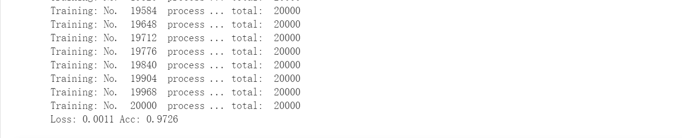
            print('Training: No. ', count, ' process ... total: ', size)
        epoch_loss = running_loss / size
        epoch_acc = running_corrects.data.item() / size
        print('Loss: {:.4f} Acc: {:.4f}'.format(
                     epoch_loss, epoch_acc))
        
        
# 模型训练
train_model(model_vgg_new,loader_train,size=dset_sizes['train'], epochs=1, 
            optimizer=optimizer_vgg)

def test_model(model,dataloader,size):
    model.eval()
    predictions = np.zeros(size)
    all_classes = np.zeros(size)
    all_proba = np.zeros((size,2))
    i = 0
    running_loss = 0.0
    running_corrects = 0
    for inputs,classes in dataloader:
        inputs = inputs.to(device)
        classes = classes.to(device)
        outputs = model(inputs)
        loss = criterion(outputs,classes)           
        _,preds = torch.max(outputs.data,1)
        # statistics
        running_loss += loss.data.item()
        running_corrects += torch.sum(preds == classes.data)
        predictions[i:i+len(classes)] = preds.to('cpu').numpy()
        all_classes[i:i+len(classes)] = classes.to('cpu').numpy()
        all_proba[i:i+len(classes),:] = outputs.data.to('cpu').numpy()
        i += len(classes)
        print('Testing: No. ', i, ' process ... total: ', size)        
    epoch_loss = running_loss / size
    epoch_acc = running_corrects.data.item() / size
    print('Loss: {:.4f} Acc: {:.4f}'.format(
                     epoch_loss, epoch_acc))
    return predictions, all_proba, all_classes

# 测试网络（valid）
predictions, all_proba, all_classes = test_model(model_vgg_new,loader_valid,size=dset_sizes['val'])

三、总结

通过这周的学习，我对卷积神经网络的有了大致的了解，知道了卷积层、池化层、全连接层的作用工作原理，还有一些经典的卷积神经网络的结构，但是就一些数学知识来说，还是没能弄懂，需要在课下补习相关的知识，对于本周的代码作业，由于刚接触没多久，只看了一部分，还有一部分没能看完，但是都尝试在colab上运行过。