Tensorflow2.0-基础
数据载体
| python:list,列表 | numpy:ndarray | tensorflow:tensor,多维数组 |
|---|---|---|
| 可使用不同数据类型,可嵌套 不连续存放, 动态指针数组 效率低,占空间大 由于高度灵活性,不适合做数值计算 |
数据类型相同 每个元素占空间相同,连续存储 占空间小,读写速度快 占用的是内存,只能在cup运算 |
可运行于gpu,tpu 支持多种计算环境 高速实现复杂算法 |
数据类型
-
tensorflow张量就是多维数组,不管是多少维的,都是张量
-
tensorflow数字默认类型:tf.int32,tf.float32,不同类型不能操作
-
numpy默认的小数是float64,
转换数据类型时:低-->高,防止数据溢出
整数转bool,0F,非零T
常用函数
-
a = tf.convert_to_tensor(numpy数据) # 将numpy数组转为tensor -
tf.is_tensor(a) #检查是否是张量 -
isinstance(a,tf.Tensor)
isinstance(a,numpy.ndarray)
特殊张量
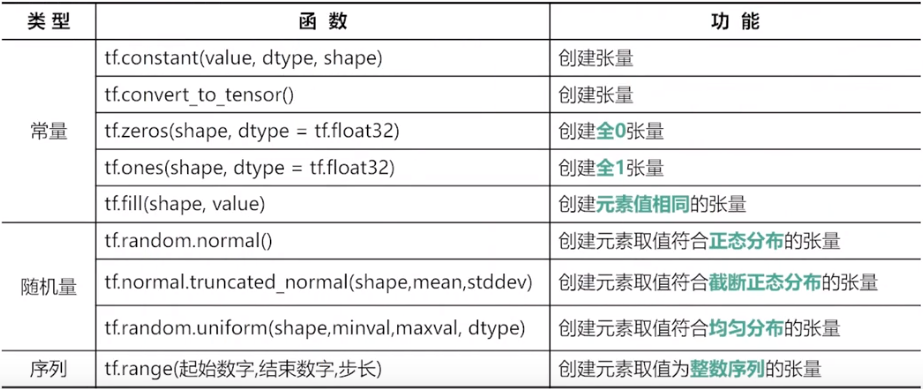
tf.zeros(shape,dtype) # 全0张量,默认是float32
tf.ones()
tf.fill(shape,value) # 自动判断数据类型,填充相同数字
tf.constant(9,[2,3]) # 也可以
tf.random.normal(shape,mean,stddev,dtype) # 正态随机分布,默认均值为0,标准差为1,float32
tf.random.truncated_normal(shape,mean,stddev,dtype)
# 截断的正态分布,截断标准是2倍标准差,值不会偏离均值2倍标准差
tf.random.uniform(shape,min,max,,type) # 均匀分布,不包含最大,包括最小
tf.random.shuffle(x) # 沿着第一维打乱
tf.random.set_seed(8) # 设置随机种子,仅仅一次有效
tf.range(start,limit,delta,dtype)# 创建序列,前闭后开,默认从0开始,步长为1
张量属性
- ndim:维度
- dtype:类型
- shape:形状
- tf.shape(a):张量形式返回形状
- tf.size(a):总数
- tf.rank(a):维度
注意
- 在cup中张量与numpy共享内存,只是使用不同方式读取使用它
- 多维张量内存中是一位数组连续存储
改变形状
b = tf.reshape(tensor,shape)
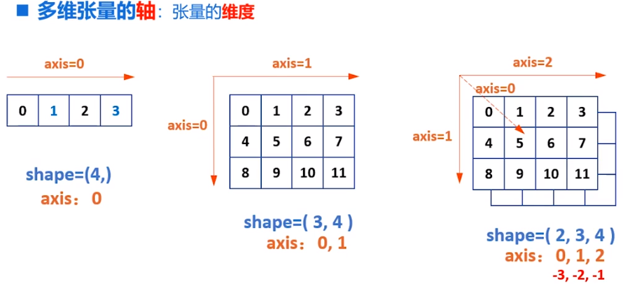
轴也可以是负数,表示从后向前
tf.expand_dims(input,axis) # 增加维度,维度长度为1
a = tf.constant([1,2]) # shape(2,)
b = tf.expand_dims(a,1) # shape(2,1) 元素数不变形状变了而已
c = tf.expand_dims(a,0) # shape(1,2)

a = tf.range(24)
b = tf.reshape(a,[2,3,4])
b1 = tf.expand_dims(b,0) # shape(1.2,3,4)
b1 = tf.expand_dims(b,1) # shape(2,1,3,4)
b1 = tf.expand_dims(b,2) # shape(2,3,1,4)
b1 = tf.expand_dims(b,3) # shape(2,3,4,1)
# 删除维度 只能删除长度为1的维度,并不会改变数量,只是改变了存储
tf.squeeze(input,axis)

a = tf.range(24)
b = tf.reshape(a,[2,1,1,3,4])
tf.squeeze(t) #shape->(2,3,4)
tf.squeeze(t,[0,1]) # shape->(1,3,4)
#交换维度,改变了视图,也改变了存储顺序
tf.transpose(a,perm)  # 对于二维张量,默认是转置
# x.shape-->(2,3)
tf.transpose(x,[1,0]) # shape->(3,2)
# 拼接,不会增加维度
tf.concat(tensor,axis) #
# 分割张量
tf.split(value,num_or_size,axis=0)
# num_or_size:2 表示平均切位2个
# [1:2:1] ,按比例切割

# 只改变视图,存储顺序不变
# 堆叠与分解
tf.stack(values,axis) #
a = tf.constant([1,2,3])
b = tf.constant([1,2,3])
tf.stack((x,y),axis=0) # shape(2,3)
tf.stack((x,y),axis=1) # shape(3,2)


tf.unstack(values,axis)
a = tf.constant([[1,2,3],[1,2,3]])
tf.stack(a,axis=0) # shape(3,) 2个
tf.stack(a,axis=1) # shape(2,) 3个
# 索引
# 与numpy几乎相同
# 一维:a[1],二维:a[1][1],a[1,1],三维:a[1][1][1],a[1,1,1]

# 切片[起始:结束:步长],步长为负数表示反向切片
# 前闭后开,起始,结束,步长可省略
# 二维数据,与一维类似,逗号隔开
# 数据提取
tf.gather(params,indices)
a = tf.range(5)
tf.gather(a,[0,2,3]) # 从a中提取0,2,3下标的元素

a = tf.random.normal([4,5])
tf.gather(a,axis=0,[0,2,3]) # 去获取0 2 3行
tf.gather(a,axis=1,[0,2,3]) # 去获取0 2 3列
# 每次只有一个维度
# 多维获取
tf.gather_nd(b,[[0,0],[1,1],[2,3]]) # 指定每个元素坐标
tf.gather_nd(三维元素,[[0,0],[1,1],[2,3]]) # 指定每个元素坐标,此时采样的是三个点,每个点三个通道
tf.gather_nd(三维元素,[[0],[1],[2]]) # 类似获取三个面
深度学习
一元线性回归
-
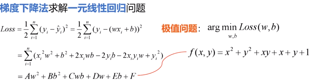
平均损失函数:\(Loss=\frac{1}{2}\mathop{\sum}\limits_{i=1}^{n}(y_i-\bar{y_i})^2=\frac{1}{2}\mathop{\sum}\limits_{i=1}^{n}(y_i-(wx_i+b))^2\)
-
均方误差:\(Loss=\frac{1}{2n}\mathop{\sum}\limits_{i=1}^{n}(y_i-\bar{y_i})^2\)
- \(\frac{1}{2}\)是为了求导方便,
- 使用平方做误差,防止正负误差抵消
- 此时Loss与误差单调性相同
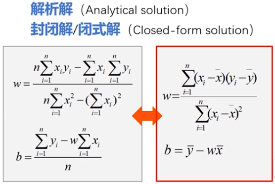
基于均方误差最小化求解模型的方法:最小二乘法
w,b作为自变量,取何值时,Loss最小?,求极值问题:极值点偏导数为0
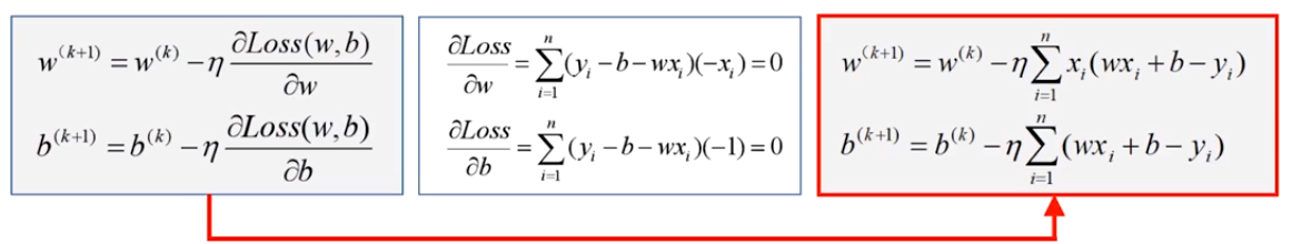
\(\frac{\partial Loss}{\partial w}=\mathop{\sum}\limits_{i=1}^{n}(y_i-b-w_i)(-x_i)=0\)
\(\frac{\partial Loss}{\partial b}=\mathop{\sum}\limits_{i=1}^{n}(y_i-b-w_i)(-1)=0\)
梯度下降
- 解析解:严格推导得出,任意精度满足方程
- 数值解:近似计算得到,给定精度下满足方程
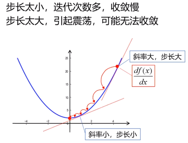
\(步长=\eta \frac{df(x)}{dx},\eta:学习率\)
\(x^{(k+1)}=x^k-步长\)
- 根据斜率实现自适应调整步长
- 自动确定下一次方向
- 保证收敛性
二元凸函数类似:
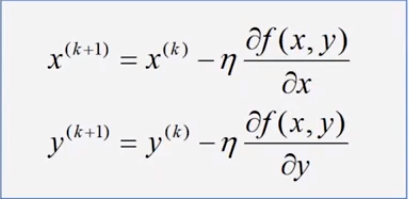
梯度:\(\vec{gard}f(x,y)=\frac{\partial f(x,y)}{\partial x}\vec{i}+\frac{\partial f(x,y)}{\partial y}\vec{j}\)
只要损失函数是凸函数,就可以使用梯度下降法,最快速度更新w,得到极值点,
凹凸性定义国内外方式不同,很可能相反
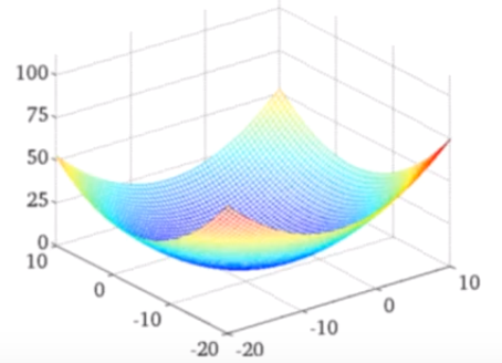
对于凸函数,只要学习率足够小,可以一定收敛,但极大会震荡,极小会很难收敛
超参数:开始先定义的
示例:
import numpy as np
import matplotlib.pyplot as plt
x = np.array([137.97,104.50,100.00,124.32,79.20,99.00,124.00,114.00,106.69,138.05,53.75,46.91,68.00,63.02,81.26,86.21])
y = np.array([145.00,110.00,93.00,116.00,65.32,104.00,118.00,91.00,62.00,133.00,51.00,45.00,78.50,69.65,75.69,95.30])
learning_rate=0.00001
iter=100
display_step=10
mse=[]
for i in range(0,iter+1):
# 计算偏导数,根据导数公式带入数据即可
dL_dw=np.mean(x*(w*x+b-y))
dL_db=np.mean(w*x+b-y)
w=w-learning_rate*dL_dw
b=b-learning_rate*dL_db
pred=w*x+b
Loss=np.mean(np.square(y-pred))/2
mse.append(Loss)
if i %display_step==0:
print("i:%i,Loss:%f,w:%f,b:%f"%(i,mse[i],w,b))
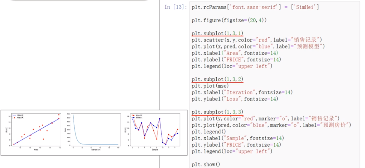
plt.rcParams['font.sans-serif']=['SimHei']
plt.figure()
plt.scatter(x,y,color='red',label="销售记录")
plt.scatter(x,pred,color="blue",label="梯度下降法")
plt.plot(x,pred,color="blue")
plt.plot(x,0.89*x+5.41,color="red")
plt.xlabel("Area",fontsize=14)
plt.ylabel("Price",fontsize=14)
plt.legend(loc="upper left")
plt.show()
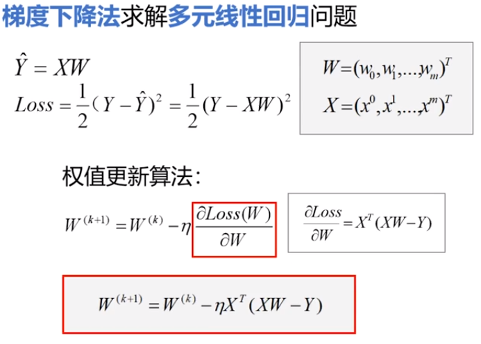
多元例子
数据归一化/标准化:将数值限制在范围内,防止某个属性影响过大
线性归一化:\(x*=\frac{x-min}{max-min}\)等比例缩放[0,1]
标准归一化:\(x*=\frac{x-\mu}{\sigma}\),归一化均值为0,方差为1,
非线性归一化:对数,指数,正切
根据数据确定
dL_dw=np.matmul(np.transpose(X),np.matmul(X,W)-Y)
W=W-lrarning_rate*dL_dW
pred =np.matmul(X,W)
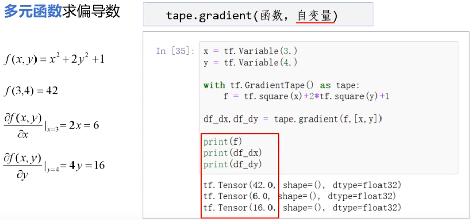
自动求导
tf.Variavle()可训练变量,可修改,有assign(),assgin_add()等,x.trainable属性等
tf.constant不同,是不可修改的
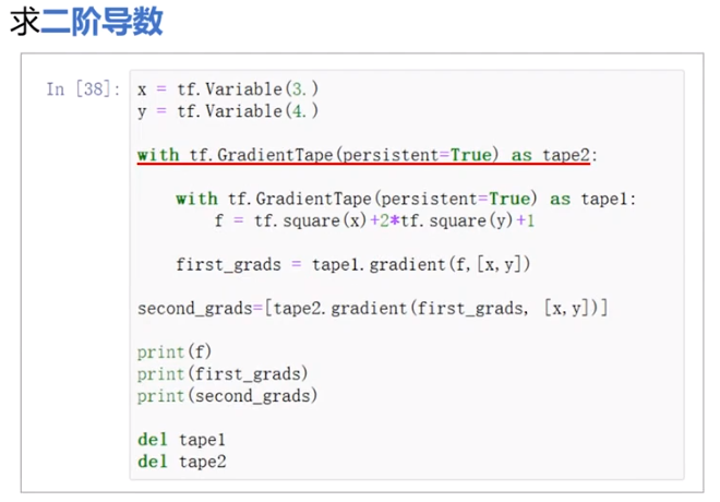
with GradienTape(persistent=True,watch_access_variables=Flase) as tape:
    tape.watch(x)
    y=tf.square(x)
grad=tape.gradient('函数','自变量') #
# persistent 为true可多次调用gradient
# 	为True时最后要 del tape
# watch默认为True,为False时需要手动watch变量

 浙公网安备 33010602011771号