吴恩达深度学习笔记 course4 week2 作业1
这周新使用了一个新框架,它是一个比较高级的框架,比起低级框架有更多的限制
使用keras要注意的是:
1.Keras框架使用的变量名和我们以前使用的numpy和TensorFlow变量不一样。它不是在前向传播的每一步上创建新变量(比如X, Z1, A1, Z2, A2,…)以便于不同层之间的计算。在Keras中,我们使用X覆盖了所有的值,没有保存每一层结果,我们只需要最新的值,唯一例外的就是X_input,我们将它分离出来是因为它是输入的数据,我们要在最后的创建模型那一步中用到。
Keras tutorial - the Happy House
Welcome to the first assignment of week 2. In this assignment, you will:
- Learn to use Keras, a high-level neural networks API (programming framework), written in Python and capable of running on top of several lower-level frameworks including TensorFlow and CNTK.
- See how you can in a couple of hours build a deep learning algorithm.
Why are we using Keras? Keras was developed to enable deep learning engineers to build and experiment with different models very quickly. Just as TensorFlow is a higher-level framework than Python, Keras is an even higher-level framework and provides additional abstractions. Being able to go from idea to result with the least possible delay is key to finding good models. However, Keras is more restrictive than the lower-level frameworks, so there are some very complex models that you can implement in TensorFlow but not (without more difficulty) in Keras. That being said, Keras will work fine for many common models.
In this exercise, you'll work on the "Happy House" problem, which we'll explain below. Let's load the required packages and solve the problem of the Happy House!
import numpy as np
from keras import layers
from keras.layers import Input, Dense, Activation, ZeroPadding2D, BatchNormalization, Flatten, Conv2D
from keras.layers import AveragePooling2D, MaxPooling2D, Dropout, GlobalMaxPooling2D, GlobalAveragePooling2D
from keras.models import Model
from keras.preprocessing import image
from keras.utils import layer_utils
from keras.utils.data_utils import get_file
from keras.applications.imagenet_utils import preprocess_input
import pydot
from IPython.display import SVG
from keras.utils.vis_utils import model_to_dot
from keras.utils import plot_model
from kt_utils import *
import keras.backend as K
K.set_image_data_format('channels_last')
import matplotlib.pyplot as plt
from matplotlib.pyplot import imshow
%matplotlib inline
Note: As you can see, we've imported a lot of functions from Keras. You can use them easily just by calling them directly in the notebook. Ex: X = Input(...) or X = ZeroPadding2D(...).
1 - The Happy House
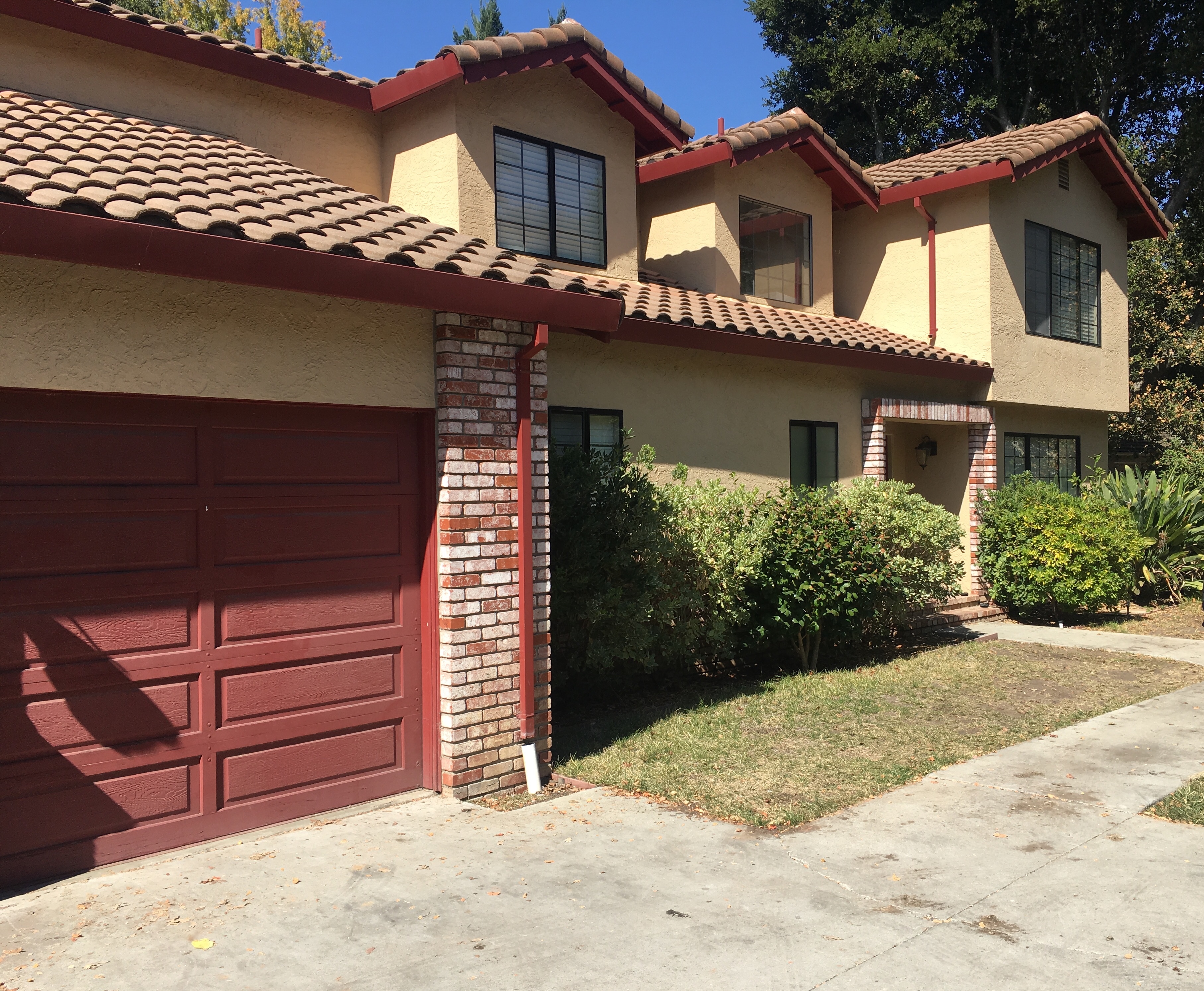
For your next vacation, you decided to spend a week with five of your friends from school. It is a very convenient house with many things to do nearby. But the most important benefit is that everybody has commited to be happy when they are in the house. So anyone wanting to enter the house must prove their current state of happiness.

As a deep learning expert, to make sure the "Happy" rule is strictly applied, you are going to build an algorithm which that uses pictures from the front door camera to check if the person is happy or not. The door should open only if the person is happy.
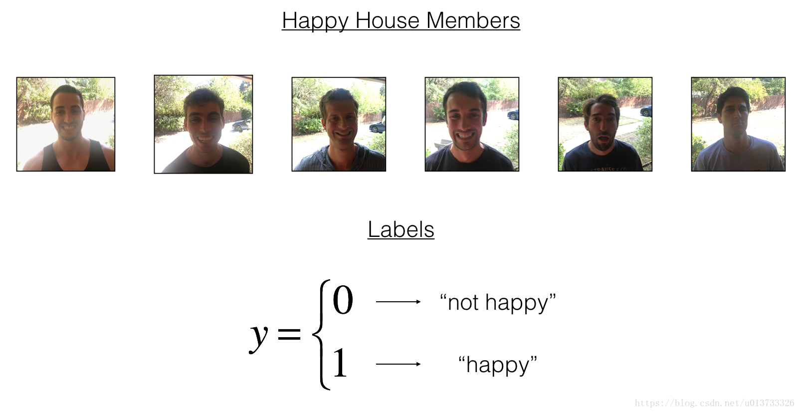
You have gathered pictures of your friends and yourself, taken by the front-door camera. The dataset is labbeled.

Run the following code to normalize the dataset and learn about its shapes.
X_train_orig, Y_train_orig, X_test_orig, Y_test_orig, classes = load_dataset()
# Normalize image vectors
X_train = X_train_orig/255.
X_test = X_test_orig/255.
# Reshape
Y_train = Y_train_orig.T
Y_test = Y_test_orig.T
print ("number of training examples = " + str(X_train.shape[0]))
print ("number of test examples = " + str(X_test.shape[0]))
print ("X_train shape: " + str(X_train.shape))
print ("Y_train shape: " + str(Y_train.shape))
print ("X_test shape: " + str(X_test.shape))
print ("Y_test shape: " + str(Y_test.shape))
Details of the "Happy" dataset:
- Images are of shape (64,64,3)
- Training: 600 pictures
- Test: 150 pictures
It is now time to solve the "Happy" Challenge.
2 - Building a model in Keras
Keras is very good for rapid prototyping. In just a short time you will be able to build a model that achieves outstanding results.
Here is an example of a model in Keras:
def model(input_shape):
# Define the input placeholder as a tensor with shape input_shape. Think of this as your input image!
X_input = Input(input_shape)
# Zero-Padding: pads the border of X_input with zeroes
X = ZeroPadding2D((3, 3))(X_input)
# CONV -> BN -> RELU Block applied to X
X = Conv2D(32, (7, 7), strides = (1, 1), name = 'conv0')(X)
X = BatchNormalization(axis = 3, name = 'bn0')(X)
X = Activation('relu')(X)
# MAXPOOL
X = MaxPooling2D((2, 2), name='max_pool')(X)
# FLATTEN X (means convert it to a vector) + FULLYCONNECTED
X = Flatten()(X)
X = Dense(1, activation='sigmoid', name='fc')(X)
# Create model. This creates your Keras model instance, you'll use this instance to train/test the model.
model = Model(inputs = X_input, outputs = X, name='HappyModel')
return model
Note that Keras uses a different convention with variable names than we've previously used with numpy and TensorFlow. In particular, rather than creating and assigning a new variable on each step of forward propagation such as X, Z1, A1, Z2, A2, etc. for the computations for the different layers, in Keras code each line above just reassigns X to a new value using X = .... In other words, during each step of forward propagation, we are just writing the latest value in the commputation into the same variable X. The only exception was X_input, which we kept separate and did not overwrite, since we needed it at the end to create the Keras model instance (model = Model(inputs = X_input, ...) above).
Exercise: Implement a HappyModel(). This assignment is more open-ended than most. We suggest that you start by implementing a model using the architecture we suggest, and run through the rest of this assignment using that as your initial model. But after that, come back and take initiative to try out other model architectures. For example, you might take inspiration from the model above, but then vary the network architecture and hyperparameters however you wish. You can also use other functions such as AveragePooling2D(), GlobalMaxPooling2D(), Dropout().
Note: You have to be careful with your data's shapes. Use what you've learned in the videos to make sure your convolutional, pooling and fully-connected layers are adapted to the volumes you're applying it to.
# GRADED FUNCTION: HappyModel
def HappyModel(input_shape):
"""
Implementation of the HappyModel.
Arguments:
input_shape -- shape of the images of the dataset
Returns:
model -- a Model() instance in Keras
"""
### START CODE HERE ###
# Feel free to use the suggested outline in the text above to get started, and run through the whole
# exercise (including the later portions of this notebook) once. The come back also try out other
# network architectures as well.
# Define the input placeholder as a tensor with shape input_shape. Think of this as your input image!
X_input = Input(input_shape)
# Zero-Padding: pads the border of X_input with zeroes
X = ZeroPadding2D((3, 3))(X_input)
# CONV -> BN -> RELU Block applied to X
X = Conv2D(32, (7, 7), strides = (1, 1), name = 'conv0')(X)
X = BatchNormalization(axis = 3, name = 'bn0')(X)
X = Activation('relu')(X)
# MAXPOOL
X = MaxPooling2D((2, 2), name='max_pool')(X)
# FLATTEN X (means convert it to a vector) + FULLYCONNECTED
X = Flatten()(X)
X = Dense(1, activation='sigmoid', name='fc')(X)
# Create model. This creates your Keras model instance, you'll use this instance to train/test the model.
model = Model(inputs = X_input, outputs = X, name='HappyModel')
### END CODE HERE ###
return model
You have now built a function to describe your model. To train and test this model, there are four steps in Keras:
- Create the model by calling the function above
- Compile the model by calling
model.compile(optimizer = "...", loss = "...", metrics = ["accuracy"]) - Train the model on train data by calling
model.fit(x = ..., y = ..., epochs = ..., batch_size = ...) - Test the model on test data by calling
model.evaluate(x = ..., y = ...)
If you want to know more about model.compile(), model.fit(), model.evaluate() and their arguments, refer to the official Keras documentation.
Exercise: Implement step 1, i.e. create the model.
### START CODE HERE ### (1 line)
happyModel = HappyModel(X_train.shape[1:])
### END CODE HERE ###
Exercise: Implement step 2, i.e. compile the model to configure the learning process. Choose the 3 arguments of compile() wisely. Hint: the Happy Challenge is a binary classification problem.
### START CODE HERE ### (1 line)
happyModel.compile("Adam","binary_crossentropy",metrics = ["accuracy"])
### END CODE HERE ###
Exercise: Implement step 3, i.e. train the model. Choose the number of epochs and the batch size.
### START CODE HERE ### (1 line)
happyModel.fit(x=X_train ,y= Y_train, epochs=30 ,batch_size=64)
### END CODE HERE ###
Note that if you run fit() again, the model will continue to train with the parameters it has already learnt instead of reinitializing them.
Exercise: Implement step 4, i.e. test/evaluate the model.
### START CODE HERE ### (1 line)
preds = happyModel.evaluate(x =X_test,y=Y_test)
### END CODE HERE ###
print()
print ("Loss = " + str(preds[0]))
print ("Test Accuracy = " + str(preds[1]))
If your happyModel() function worked, you should have observed much better than random-guessing (50%) accuracy on the train and test sets.
To give you a point of comparison, our model gets around 95% test accuracy in 40 epochs (and 99% train accuracy) with a mini batch size of 16 and "adam" optimizer. But our model gets decent accuracy after just 2-5 epochs, so if you're comparing different models you can also train a variety of models on just a few epochs and see how they compare.
If you have not yet achieved a very good accuracy (let's say more than 80%), here're some things you can play around with to try to achieve it:
- Try using blocks of CONV->BATCHNORM->RELU such as:
until your height and width dimensions are quite low and your number of channels quite large (≈32 for example). You are encoding useful information in a volume with a lot of channels. You can then flatten the volume and use a fully-connected layer.X = Conv2D(32, (3, 3), strides = (1, 1), name = 'conv0')(X) X = BatchNormalization(axis = 3, name = 'bn0')(X) X = Activation('relu')(X) - You can use MAXPOOL after such blocks. It will help you lower the dimension in height and width.
- Change your optimizer. We find Adam works well.
- If the model is struggling to run and you get memory issues, lower your batch_size (12 is usually a good compromise)
- Run on more epochs, until you see the train accuracy plateauing.
Even if you have achieved a good accuracy, please feel free to keep playing with your model to try to get even better results.
Note: If you perform hyperparameter tuning on your model, the test set actually becomes a dev set, and your model might end up overfitting to the test (dev) set. But just for the purpose of this assignment, we won't worry about that here.
3 - Conclusion
Congratulations, you have solved the Happy House challenge!
Now, you just need to link this model to the front-door camera of your house. We unfortunately won't go into the details of how to do that here.
What we would like you to remember from this assignment:
- Keras is a tool we recommend for rapid prototyping. It allows you to quickly try out different model architectures. Are there any applications of deep learning to your daily life that you'd like to implement using Keras?
- Remember how to code a model in Keras and the four steps leading to the evaluation of your model on the test set. Create->Compile->Fit/Train->Evaluate/Test.
4 - Test with your own image (Optional)
Congratulations on finishing this assignment. You can now take a picture of your face and see if you could enter the Happy House. To do that:
1. Click on "File" in the upper bar of this notebook, then click "Open" to go on your Coursera Hub.
2. Add your image to this Jupyter Notebook's directory, in the "images" folder
3. Write your image's name in the following code
4. Run the code and check if the algorithm is right (0 is unhappy, 1 is happy)!
The training/test sets were quite similar; for example, all the pictures were taken against the same background (since a front door camera is always mounted in the same position). This makes the problem easier, but a model trained on this data may or may not work on your own data. But feel free to give it a try!
### START CODE HERE ###
img_path = 'images/my_image.jpg'
### END CODE HERE ###
img = image.load_img(img_path, target_size=(64, 64))
imshow(img)
x = image.img_to_array(img)
x = np.expand_dims(x, axis=0)
x = preprocess_input(x)
print(happyModel.predict(x))

5 - Other useful functions in Keras (Optional)
Two other basic features of Keras that you'll find useful are:
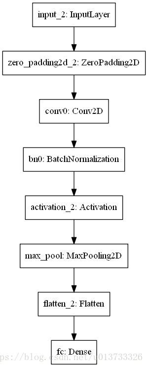
model.summary(): prints the details of your layers in a table with the sizes of its inputs/outputsplot_model(): plots your graph in a nice layout. You can even save it as ".png" using SVG() if you'd like to share it on social media ;). It is saved in "File" then "Open..." in the upper bar of the notebook.
Run the following code.
happyModel.summary()
plot_model(happyModel, to_file='HappyModel.png')
SVG(model_to_dot(happyModel).create(prog='dot', format='svg'))
资料下载
-
下载1:本文所使用的资料已上传到百度网盘【点击下载(15.97MB)】,请在开始之前下载好所需资料,或者在本文底部copy资料代码。
-
下载2(有偿下载):在残差网络中博主花费大力气训练好了残差网络的权值,这部分是需要有偿下载的,需要使用C币进行下载,下载地址:https://download.csdn.net/download/u013733326/10403196
【博主使用的python版本:3.6.2】
1 - Keras 入门 - 笑脸识别
本次我们将:
1. 学习到一个高级的神经网络的框架,能够运行在包括TensorFlow和CNTK的几个较低级别的框架之上的框架。
2. 看看如何在几个小时内建立一个深入的学习算法。
为什么我们要使用Keras框架呢?Keras是为了使深度学习工程师能够很快地建立和实验不同的模型的框架,正如TensorFlow是一个比Python更高级的框架,Keras是一个更高层次的框架,并提供了额外的抽象方法。最关键的是Keras能够以最短的时间让想法变为现实。然而,Keras比底层框架更具有限制性,所以有一些非常复杂的模型可以在TensorFlow中实现,但在Keras中却没有(没有更多困难)。 话虽如此,Keras对许多常见模型都能正常运行。
import numpy as np
from keras import layers
from keras.layers import Input, Dense, Activation, ZeroPadding2D, BatchNormalization, Flatten, Conv2D
from keras.layers import AveragePooling2D, MaxPooling2D, Dropout, GlobalMaxPooling2D, GlobalAveragePooling2D
from keras.models import Model
from keras.preprocessing import image
from keras.utils import layer_utils
from keras.utils.data_utils import get_file
from keras.applications.imagenet_utils import preprocess_input
import pydot
from IPython.display import SVG
from keras.utils.vis_utils import model_to_dot
from keras.utils import plot_model
import kt_utils
import keras.backend as K
K.set_image_data_format('channels_last')
import matplotlib.pyplot as plt
from matplotlib.pyplot import imshow
%matplotlib inline- 1
- 2
- 3
- 4
- 5
- 6
- 7
- 8
- 9
- 10
- 11
- 12
- 13
- 14
- 15
- 16
- 17
- 18
- 19
- 20
- 21
注意:正如你所看到的,我们已经从Keras中导入了很多功能, 只需直接调用它们即可轻松使用它们。 比如:X = Input(…) 或者X = ZeroPadding2D(…).
1.1 - 任务描述
下一次放假的时候,你决定和你的五个朋友一起度过一个星期。这是一个非常好的房子,在附近有很多事情要做,但最重要的好处是每个人在家里都会感到快乐,所以任何想进入房子的人都必须证明他们目前的幸福状态。
作为一个深度学习的专家,为了确保“快乐才开门”规则得到严格的应用,你将建立一个算法,它使用来自前门摄像头的图片来检查这个人是否快乐,只有在人高兴的时候,门才会打开。
你收集了你的朋友和你自己的照片,被前门的摄像头拍了下来。数据集已经标记好了。。
我们先来加载数据集:
X_train_orig, Y_train_orig, X_test_orig, Y_test_orig, classes = kt_utils load_dataset()
# Normalize image vectors
X_train = X_train_orig/255.
X_test = X_test_orig/255.
# Reshape
Y_train = Y_train_orig.T
Y_test = Y_test_orig.T
print ("number of training examples = " + str(X_train.shape[0]))
print ("number of test examples = " + str(X_test.shape[0]))
print ("X_train shape: " + str(X_train.shape))
print ("Y_train shape: " + str(Y_train.shape))
print ("X_test shape: " + str(X_test.shape))
print ("Y_test shape: " + str(Y_test.shape))- 1
- 2
- 3
- 4
- 5
- 6
- 7
- 8
- 9
- 10
- 11
- 12
- 13
- 14
- 15
- 16
执行结果:
number of training examples = 600
number of test examples = 150
X_train shape: (600, 64, 64, 3)
Y_train shape: (600, 1)
X_test shape: (150, 64, 64, 3)
Y_test shape: (150, 1)- 1
- 2
- 3
- 4
- 5
- 6
数据集的细节如下:
- 图像维度:(64,64,3)
- 训练集数量:600
- 测试集数量:150
1.2 - 使用Keras框架构建模型
Keras非常适合快速制作模型,它可以在很短的时间内建立一个很优秀的模型,举个例子:
def model(input_shape):
"""
模型大纲
"""
#定义一个tensor的placeholder,维度为input_shape
X_input = Input(input_shape)
#使用0填充:X_input的周围填充0
X = ZeroPadding2D((3,3))(X_input)
# 对X使用 CONV -> BN -> RELU 块
X = Conv2D(32, (7, 7), strides = (1, 1), name = 'conv0')(X)
X = BatchNormalization(axis = 3, name = 'bn0')(X)
X = Activation('relu')(X)
#最大值池化层
X = MaxPooling2D((2,2),name="max_pool")(X)
#降维,矩阵转化为向量 + 全连接层
X = Flatten()(X)
X = Dense(1, activation='sigmoid', name='fc')(X)
#创建模型,讲话创建一个模型的实体,我们可以用它来训练、测试。
model = Model(inputs = X_input, outputs = X, name='HappyModel')
return model
- 1
- 2
- 3
- 4
- 5
- 6
- 7
- 8
- 9
- 10
- 11
- 12
- 13
- 14
- 15
- 16
- 17
- 18
- 19
- 20
- 21
- 22
- 23
- 24
- 25
- 26
- 27
请注意:Keras框架使用的变量名和我们以前使用的numpy和TensorFlow变量不一样。它不是在前向传播的每一步上创建新变量(比如X, Z1, A1, Z2, A2,…)以便于不同层之间的计算。在Keras中,我们使用X覆盖了所有的值,没有保存每一层结果,我们只需要最新的值,唯一例外的就是X_input,我们将它分离出来是因为它是输入的数据,我们要在最后的创建模型那一步中用到。
def HappyModel(input_shape):
"""
实现一个检测笑容的模型
参数:
input_shape - 输入的数据的维度
返回:
model - 创建的Keras的模型
"""
#你可以参考和上面的大纲
X_input = Input(input_shape)
#使用0填充:X_input的周围填充0
X = ZeroPadding2D((3, 3))(X_input)
#对X使用 CONV -> BN -> RELU 块
X = Conv2D(32, (7, 7), strides=(1, 1), name='conv0')(X)
X = BatchNormalization(axis=3, name='bn0')(X)
X = Activation('relu')(X)
#最大值池化层
X = MaxPooling2D((2, 2), name='max_pool')(X)
#降维,矩阵转化为向量 + 全连接层
X = Flatten()(X)
X = Dense(1, activation='sigmoid', name='fc')(X)
#创建模型,讲话创建一个模型的实体,我们可以用它来训练、测试。
model = Model(inputs=X_input, outputs=X, name='HappyModel')
return model- 1
- 2
- 3
- 4
- 5
- 6
- 7
- 8
- 9
- 10
- 11
- 12
- 13
- 14
- 15
- 16
- 17
- 18
- 19
- 20
- 21
- 22
- 23
- 24
- 25
- 26
- 27
- 28
- 29
- 30
- 31
- 32
- 33
现在我们已经设计好了我们的模型了,要训练并测试模型我们需要这么做:
- 创建一个模型实体。
- 编译模型,可以使用这个语句:
model.compile(optimizer = "...", loss = "...", metrics = ["accuracy"])。 - 训练模型:
model.fit(x = ..., y = ..., epochs = ..., batch_size = ...)。 - 评估模型:
model.evaluate(x = ..., y = ...)。
如果你想要获取关于model.compile(), model.fit(), model.evaluate()的更多的信息,你可以参考这里。
#创建一个模型实体
happy_model = HappyModel(X_train.shape[1:])
#编译模型
happy_model.compile("adam","binary_crossentropy", metrics=['accuracy'])
#训练模型
#请注意,此操作会花费你大约6-10分钟。
happy_model.fit(X_train, Y_train, epochs=40, batch_size=50)
#评估模型
preds = happy_model.evaluate(X_test, Y_test, batch_size=32, verbose=1, sample_weight=None)
print ("误差值 = " + str(preds[0]))
print ("准确度 = " + str(preds[1]))- 1
- 2
- 3
- 4
- 5
- 6
- 7
- 8
- 9
- 10
- 11
执行结果:
Epoch 1/40
600/600 [==============================] - 12s 19ms/step - loss: 2.2593 - acc: 0.5667
Epoch 2/40
600/600 [==============================] - 9s 16ms/step - loss: 0.5355 - acc: 0.7917
Epoch 3/40
600/600 [==============================] - 10s 17ms/step - loss: 0.3252 - acc: 0.8650
Epoch 4/40
600/600 [==============================] - 10s 17ms/step - loss: 0.2038 - acc: 0.9250
Epoch 5/40
600/600 [==============================] - 10s 16ms/step - loss: 0.1664 - acc: 0.9333
...
Epoch 38/40
600/600 [==============================] - 10s 17ms/step - loss: 0.0173 - acc: 0.9950
Epoch 39/40
600/600 [==============================] - 14s 23ms/step - loss: 0.0365 - acc: 0.9883
Epoch 40/40
600/600 [==============================] - 12s 19ms/step - loss: 0.0291 - acc: 0.9900
150/150 [==============================] - 3s 21ms/step
误差值 = 0.407454126676
准确度 = 0.840000001589- 1
- 2
- 3
- 4
- 5
- 6
- 7
- 8
- 9
- 10
- 11
- 12
- 13
- 14
- 15
- 16
- 17
- 18
- 19
- 20
- 21
- 22
只要准确度大于75%就算正常,如果你的准确度没有大于75%,你可以尝试改变模型:
X = Conv2D(32, (3, 3), strides = (1, 1), name = 'conv0')(X)
X = BatchNormalization(axis = 3, name = 'bn0')(X)
X = Activation('relu')(X)- 1
- 2
- 3
- 你可以在每个块后面使用最大值池化层,它将会减少宽、高的维度。
- 改变优化器,这里我们使用的是Adam
- 如果模型难以运行,并且遇到了内存不够的问题,那么就降低batch_size(12通常是一个很好的折中方案)
- 运行更多代,直到看到有良好效果的时候。
即使你已经达到了75%的准确度,你也可以继续优化你的模型,以获得更好的结果。
1.3 - 总结
这个任务算是完成了,你可以在你家试试[手动滑稽]
1.4 - 测试你的图片
因为对这些数据进行训练的模型可能或不能处理你自己的图片,但是你可以试一试嘛:
#网上随便找的图片,侵删
img_path = 'images/smile.jpeg'

img = image.load_img(img_path, target_size=(64, 64))
imshow(img)

x = image.img_to_array(img)
x = np.expand_dims(x, axis=0)
x = preprocess_input(x)

print(happy_model.predict(x))- 1
- 2
- 3
- 4
- 5
- 6
- 7
- 8
- 9
- 10
- 11
测试结果:
[[ 1.]]- 1

img_path = 'images/my_image.jpg'

img = image.load_img(img_path, target_size=(64, 64))
imshow(img)

x = image.img_to_array(img)
x = np.expand_dims(x, axis=0)
x = preprocess_input(x)

print(happy_model.predict(x))- 1
- 2
- 3
- 4
- 5
- 6
- 7
- 8
- 9
- 10
测试结果:
[[ 0.]]- 1

1.5 - 其他一些有用的功能
model.summary():打印出你的每一层的大小细节plot_model(): 绘制出布局图
happy_model.summary()- 1
执行结果:
_________________________________________________________________
Layer (type)                 Output Shape              Param #
=================================================================
input_2 (InputLayer)         (None, 64, 64, 3)         0
_________________________________________________________________
zero_padding2d_2 (ZeroPaddin (None, 70, 70, 3)         0
_________________________________________________________________
conv0 (Conv2D)               (None, 64, 64, 32)        4736
_________________________________________________________________
bn0 (BatchNormalization)     (None, 64, 64, 32)        128
_________________________________________________________________
activation_2 (Activation)    (None, 64, 64, 32)        0
_________________________________________________________________
max_pool (MaxPooling2D)      (None, 32, 32, 32)        0
_________________________________________________________________
flatten_2 (Flatten)          (None, 32768)             0
_________________________________________________________________
fc (Dense)                   (None, 1)                 32769
=================================================================
Total params: 37,633
Trainable params: 37,569
Non-trainable params: 64
_________________________________________________________________- 1
- 2
- 3
- 4
- 5
- 6
- 7
- 8
- 9
- 10
- 11
- 12
- 13
- 14
- 15
- 16
- 17
- 18
- 19
- 20
- 21
- 22
- 23
我们来绘制一下图:
天坑:
1. 请下载并安装Graphviz的windows版本,然后写入环境变量,博主的环境变量填的是:E:\Anaconda3\Lib\site-packages\Graphviz\bin,因人而异吧.
2. 请安装pydot-ng & graphviz,其代码CMD代码为:pip install pydot-ng & pip install graphviz或者是pip install pydot 与 pip install graphviz
3. 重启Jupyter Notebook 【手动微笑】【手动再见】
%matplotlib inline
plot_model(happy_model, to_file='happy_model.png')
SVG(model_to_dot(happy_model).create(prog='dot', format='svg'))- 1
- 2
- 3

 浙公网安备 33010602011771号