吴恩达深度学习笔记（六） —— 卷积神经网络

 

 

主要内容：

一.卷积神经网络简介

二.卷积神经网络之前向传播简介

三.padding填充

四.stride步长

五.信道(channel)个数与过滤器(filter)个数的区别

六.卷积的一步

七.一次完整的卷积

八.池化层

九.1 * 1 filter

 

 

一.卷积神经网络介绍

1.何为卷积神经网络？顾名思义，就是在神经网络上引入了卷积思想，以此实现了参数共享、大大地降低的参数的数量规模。尤其是在计算机视觉方面，由于一张图片由数以万计的像素组成，如果为每个像素点（作为输入层X）与下一层的结点的相连之处都配置一个参数，那么参数的个数是非常巨大，尤其是在深层神经网络上，如此一来，计算成本将十分巨大。但在卷积神经网络中，引入了过滤器，过滤器实际上就是一个以矩阵或矩阵队列形式出现的参数集合，过滤器往往比输入的像素矩阵小很多。

2.在计算机视觉方面，通常要做的就是边界检测，由于边界一般都拥有共性，更直接地说是：对于边界区域，他们的参数是相似的，既然相似就可以去除冗余，把共性的东西抽取出来，这便是过滤器。所以过滤器在感性层面上的工作就是边界检测。

3.由于卷积神经网络的反向传播比较复杂，且诸如tensorflow的框架已经帮我们实现了反向传播，因此就不谈论反向传播的问题。

 

 

二.卷积神经网络之前向传播简介

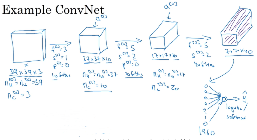
1）首先输入一张图像，可以使RGB图像，即 n_H * n_W * n_C 的结构，其中n_H 、n_W为高和宽，n_C为信道数，RGB图像由三种叠加在一起，所以n_C为3。

2）之后输入数据被若干个过滤器进行卷积，假设有k个过滤器，一个过滤器的结构为 f *f * n_C，其中f为宽和高，n_C为信道数，过滤器的信道数必须与它卷积的对象的信道数保持一致，否则匹配不成功无法进行卷积，因此这里n_C为3。一个过滤器卷积一步就形成一个数（对应位置的元素相乘然后求和），一个过滤器卷积完就形成一个n_new_H * n_new_W的矩阵，然后把k个过滤器卷积得到的k个矩阵叠加在一起，就形成了一个n_new_H * n_new_W * k 的矩体，其中k就是新的信道，因此又可以写成n_new_H * n_new_W * n_new_C。这个矩体就作为下一层的输入。

3）将卷积层的输出输入到激活函数如Relu()中，输出作为下一层的输入。

4）将上一层的输出输入到一个池化层，池化层的目的主要是缩短输入的宽和高，减少计算量。一般地有max pooling和average pooling。

5）到达最后一层时，将输入从原来的矩体摊开成一条队列，即回归到普通神经网络那样，一层就是一条及结点队列。之后用这一层结点与下一层的结点做全连接，下一层的输入经过处理如softmax处理之后，就可以作为一次前向传播的最终输出了。

 

 

三.padding填充

1.在卷积的过程中，如果不对输入的边界进行一定的填充，那么每一层的输入就会越卷越小。同时，由于输入边界的数据被过滤器滑过的次数较输入内部数据的次数少，导致了边界信息丢失。为了解决这两个问题，可以在进行卷积之前对输入进行填充。

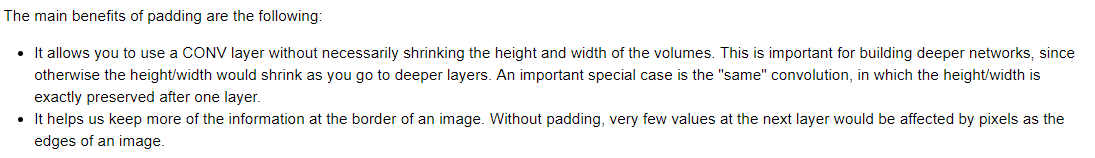
2.一般地，有zero-padding，即使得卷积前后的宽和高保持不变。注意：填充并不能保持信道不变，因为信道是由过滤器的个数决定的。

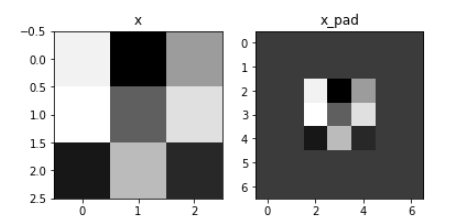
# GRADED FUNCTION: zero_pad

def zero_pad(X, pad):
    """
    Pad with zeros all images of the dataset X. The padding is applied to the height and width of an image, 
    as illustrated in Figure 1.
    
    Argument:
    X -- python numpy array of shape (m, n_H, n_W, n_C) representing a batch of m images
    pad -- integer, amount of padding around each image on vertical and horizontal dimensions
    
    Returns:
    X_pad -- padded image of shape (m, n_H + 2*pad, n_W + 2*pad, n_C)
    """
    
    ### START CODE HERE ### (≈ 1 line)
    X_pad = np.pad(X, ((0, 0), (pad, pad), (pad, pad), (0, 0)), 'constant', constant_values=0)
    ### END CODE HERE ###
    
    return X_pad

 

 

 

四.stride步长

1.当过滤器在当前位置卷积完后，下一个卷积位置要夸多少个格式可以调的，也就是所谓的步长stride。可知，当步长越小，对数据考虑地越精细，保存的信息越多；步长越大，则考虑得粗略，保存的数据少。

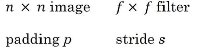
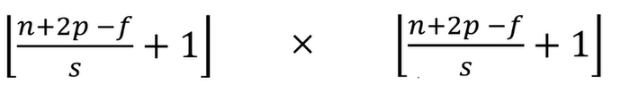
2.步长不同，相同的数据和过滤器所卷积出来的结果的宽和高也不同，其基三公式如下：

 

 

五.信道(channel)个数与过滤器(filter)个数

1.上一层输出的矩体为 n_H * n_W * n_C，所以其信道个数为n_C。假设卷积层有k个过滤器，对于一个过滤器，为了能够与矩体卷积，这个过滤器的信道也必须为n_C，所以过滤器的结构为 f * f * n_C。

2.一个过滤器卷积完就形成一个n_new_H * n_new_W的矩阵，然后把k个过滤器卷积得到的k个矩阵叠加在一起，就形成了一个n_new_H * n_new_W * k 的矩体，其中k就是新的信道，因此又可以写成n_new_H * n_new_W * n_new_C。这个矩体就作为下层的输入，以此循环下去。

3.总结：上一层输出的信道数等于过滤器的信道数，而过滤器的个数又作为这一层输出的信道数。

 

 

六.卷积的一步

这里说的“卷积的一步”，指的是一个过滤器在矩体某一位置的卷积。其卷积结果是一个实数，计算方式为：对应位置相乘然后求和，最后再加上一个偏移值b（一个过滤器一个偏移值b）。

代码如下：

# GRADED FUNCTION: conv_single_step
def conv_single_step(a_slice_prev, W, b):
    """
    Apply one filter defined by parameters W on a single slice (a_slice_prev) of the output activation 
    of the previous layer.
    
    Arguments:
    a_slice_prev -- slice of input data of shape (f, f, n_C_prev)
    W -- Weight parameters contained in a window - matrix of shape (f, f, n_C_prev)
    b -- Bias parameters contained in a window - matrix of shape (1, 1, 1)
    
    Returns:
    Z -- a scalar value, result of convolving the sliding window (W, b) on a slice x of the input data
    """

    ### START CODE HERE ### (≈ 2 lines of code)
    # Element-wise product between a_slice and W. Do not add the bias yet.
    s = a_slice_prev * W
    # Sum over all entries of the volume s.
    Z = np.sum(s)
    # Add bias b to Z. Cast b to a float() so that Z results in a scalar value.
    Z = Z + float(b)
    ### END CODE HERE ###
    return Z

 

 

七.一次完整的卷积

1.所谓“一次完成的卷积”，即是：一个矩体输入到卷积层，经过若干个过滤器的处理后，输出一个新矩体的过程。

2.做法是：每个过滤器轮流对输入矩体作卷积，然后将得到的矩形堆叠在一起，形成新的矩体。

代码如下：

# GRADED FUNCTION: conv_forward

def conv_forward(A_prev, W, b, hparameters):
    """
    Implements the forward propagation for a convolution function
    
    Arguments:
    A_prev -- output activations of the previous layer, numpy array of shape (m, n_H_prev, n_W_prev, n_C_prev)
    W -- Weights, numpy array of shape (f, f, n_C_prev, n_C)
    b -- Biases, numpy array of shape (1, 1, 1, n_C)
    hparameters -- python dictionary containing "stride" and "pad"
        
    Returns:
    Z -- conv output, numpy array of shape (m, n_H, n_W, n_C)
    cache -- cache of values needed for the conv_backward() function
    """
    
    ### START CODE HERE ###
    # Retrieve dimensions from A_prev's shape (≈1 line)  
    (m, n_H_prev, n_W_prev, n_C_prev) = A_prev.shape
    
    # Retrieve dimensions from W's shape (≈1 line)
    (f, f, n_C_prev, n_C) = W.shape
    
    # Retrieve information from "hparameters" (≈2 lines)
    stride = hparameters['stride']
    pad = hparameters['pad']
    
    # Compute the dimensions of the CONV output volume using the formula given above. Hint: use int() to floor. (≈2 lines)
    n_H = int((n_H_prev-f+2*pad)/stride)+1
    n_W = int((n_W_prev-f+2*pad)/stride)+1
    
    # Initialize the output volume Z with zeros. (≈1 line)
    Z = np.zeros((m,n_H,n_W,n_C))
    
    # Create A_prev_pad by padding A_prev
    A_prev_pad = zero_pad(A_prev,pad)
    
    for i in range(m):                               # loop over the batch of training examples
        a_prev_pad = A_prev_pad[i]                               # Select ith training example's padded activation
        for h in range(n_H):                           # loop over vertical axis of the output volume
            for w in range(n_W):                       # loop over horizontal axis of the output volume
                for c in range(n_C):                   # loop over channels (= #filters) of the output volume
                    
                    # Find the corners of the current "slice" (≈4 lines)
                    vert_start = h * stride
                    vert_end = vert_start + f
                    horiz_start = w * stride
                    horiz_end = horiz_start + f
                    
                    # Use the corners to define the (3D) slice of a_prev_pad (See Hint above the cell). (≈1 line)
                    a_slice_prev = a_prev_pad[vert_start:vert_end, horiz_start:horiz_end]
                    
                    # Convolve the (3D) slice with the correct filter W and bias b, to get back one output neuron. (≈1 line)
                    Z[i, h, w, c] = conv_single_step(a_slice_prev,W[...,c],b[...,c])
                                        
    ### END CODE HERE ###
    
    # Making sure your output shape is correct
    assert(Z.shape == (m, n_H, n_W, n_C))
    
    # Save information in "cache" for the backprop
    cache = (A_prev, W, b, hparameters)
    
    return Z, cache

 

 

八.池化层

The pooling (POOL) layer reduces the height and width of the input. It helps reduce computation, as well as helps make feature detectors more invariant to its position in the input. The two types of pooling layers are:

1）Max-pooling layer: slides an f * f window over the input and stores the max value of the window in the output.

2）Average-pooling layer: slides an f * f window over the input and stores the average value of the window in the output.

3）These pooling layers have no parameters for backpropagation to train. However, they have hyperparameters such as the window size f. This specifies the height and width of the fxf window you would compute a max or average over.

代码如下：

# GRADED FUNCTION: pool_forward

def pool_forward(A_prev, hparameters, mode = "max"):
    """
    Implements the forward pass of the pooling layer
    
    Arguments:
    A_prev -- Input data, numpy array of shape (m, n_H_prev, n_W_prev, n_C_prev)
    hparameters -- python dictionary containing "f" and "stride"
    mode -- the pooling mode you would like to use, defined as a string ("max" or "average")
    
    Returns:
    A -- output of the pool layer, a numpy array of shape (m, n_H, n_W, n_C)
    cache -- cache used in the backward pass of the pooling layer, contains the input and hparameters 
    """
    
    # Retrieve dimensions from the input shape
    (m, n_H_prev, n_W_prev, n_C_prev) = A_prev.shape
    
    # Retrieve hyperparameters from "hparameters"
    f = hparameters["f"]
    stride = hparameters["stride"]
    
    # Define the dimensions of the output
    n_H = int(1 + (n_H_prev - f) / stride)
    n_W = int(1 + (n_W_prev - f) / stride)
    n_C = n_C_prev
    
    # Initialize output matrix A
    A = np.zeros((m, n_H, n_W, n_C))              
    
    ### START CODE HERE ###
    for i in range(m):                         # loop over the training examples
        for h in range(n_H):                     # loop on the vertical axis of the output volume
            for w in range(n_W):                 # loop on the horizontal axis of the output volume
                for c in range (n_C):            # loop over the channels of the output volume
                    
                    # Find the corners of the current "slice" (≈4 lines)
                    vert_start = stride * h
                    vert_end = vert_start + f
                    horiz_start = stride * w
                    horiz_end = horiz_start + f
                    
                    # Use the corners to define the current slice on the ith training example of A_prev, channel c. (≈1 line)
                    a_prev_slice = A_prev[i,vert_start:vert_end,horiz_start:horiz_end,c]
                    
                    # Compute the pooling operation on the slice. Use an if statment to differentiate the modes. Use np.max/np.mean.
                    if mode == "max":
                        A[i, h, w, c] = np.max(a_prev_slice)
                    elif mode == "average":
                        A[i, h, w, c] = np.mean(a_prev_slice)
    
    ### END CODE HERE ###
    
    # Store the input and hparameters in "cache" for pool_backward()
    cache = (A_prev, hparameters)
    
    # Making sure your output shape is correct
    assert(A.shape == (m, n_H, n_W, n_C))
    
    return A, cache

 

 

九.1 * 1 filter

如果说，池化层的作用是用来调整n_W和n_H，那么1 * 1，准确而言，是n_new_C个1 * 1 * n_C的过滤器的作用是调节信道数：