NICE: NON-LINEAR INDEPENDENT COMPONENTS ESTIMATION

一. 基本思想

文章将图像通过 f(x) 映射到一个新的潜在向量空间中,并通过修改潜在向量经过 f(x)逆变换得到修改后的图像。为了实现该想法，需要保证在变换过程中的雅可比行列式计算和逆运算方便，NICE提出了Coupling layer 模块。

Coupling layer

• 基本实现

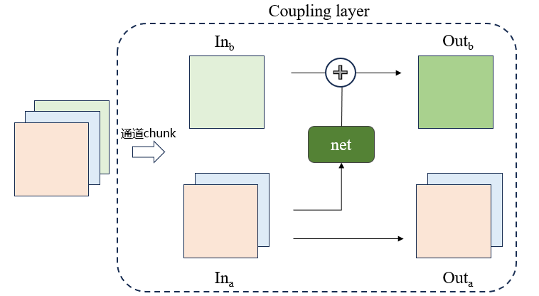
  将输入分为两个部分 x_1, x_2 (通道拆分),x_1不经过变换直接输出y_1, x_2 经过变换输出 y_2, 变换公式如下所示:

  \[f(x) = \begin{cases} y_1 = x_1\\ y_2 = m(x1)+x_2\\ \end{cases} \]

该变换的雅可比矩阵容易计算,如下所示,可以发现,无论m变换多么复杂,该变换的雅可比矩阵值行列式的值都为1.

\[\begin{Vmatrix} \frac{\partial y_1}{\partial x1}& \frac{\partial y_1}{\partial x2}\\ \frac{\partial y_2}{\partial x1}& \frac{\partial y_2}{\partial x2}\\ \end{Vmatrix} =\begin{Vmatrix} I_d&0\\ \frac{\partial y_2}{\partial x1}&I_{D-d}\\ \end{Vmatrix} \]

逆运算：

\[ \begin{cases} x_1 = y_1\\ x_2 = y_2-m(y_1)\\ \end{cases} \]

• 代码（pytorch简单实现）

import torch
import torch.nn as nn
class CouplingLayer(nn.Module):
    def __init__(self, inChannel, filter_size):
        super().__init__()

        self.net = nn.Sequential(
            nn.Conv2d(inChannel - inChannel // 2, filter_size, 3, padding=1),
            nn.Conv2d(filter_size, inChannel // 2, 1),
        )
    def forward(self, input):
        in_a, in_b = input.chunk(2, 1) # 通道拆分
        out_a = in_a
        out_b = self.net(in_a) + in_b
        out = torch.cat([out_a, out_b], dim = 1)
        return out

    def reverse(self, output):
        out_a, out_b = output.chunk(2, 1)
        in_a = out_a
        in_b = out_b - self.net(out_a)
        in_ = torch.cat([in_a, in_b], dim=1)
        return in_

model = CouplingLayer(3, 12)
inputs = torch.randn(4,3,224,224) #(b c h w)
outputs = model(inputs)
reversed_inputs = model.reverse(outputs)

# 检查输出和逆的维度
print(outputs.shape)
print(reversed_inputs.shape)
print(torch.allclose(inputs, reversed_inputs, atol=1e-6)) #表示反向还原成功

• 存在的问题

  • 始终有一部分的通道不参与变换
  • Coupling layer的行列式矩阵值始终为1，在log变换为0，对于目标函数（详见第二章）来说并不起到任何作用

​ 为了实现不同的通道参与变换，在实现过程中通过交替变换的方式，例如第 i + 1 层是in_a变换，那么第 i 层就是in_a不变，in_b变换。除此之外，为了获得更多的权重参数，在最后一层Coupling layer后加入可学习Scaling module的缩放因子矩阵S，由于Coupling layer的雅可比矩阵始终为 I，因此最后得到的输出结果为diag S

\[\begin{bmatrix} s_{11}&0\\ 0&s_{22}\\ \end{bmatrix} \]

Scaling module 代码实现

class Scaling(nn.Module):
    def __init__(self, dim):
        super(Scaling, self).__init__()
        self.scale = nn.Parameter(
            torch.zeros((1, dim)), requires_grad=True)

    def forward(self, x):
        log_det_J = torch.sum(self.scale) * x.shape[0] #相当于在每一层上都进行了缩放
        x = x * torch.exp(self.scale)
        return x, log_det_J
    
   	def reverse(self, x):
        log_det_J = torch.sum(self.scale) * x.shape[0] 
        x = x * torch.exp(-self.scale)
        return x, log_det_J

二. 数学原理

​ 原图像通过 f(x) 映射到h空间中,可以记为:

\[h = f(x) \]

​ 从而当修改潜在空间向量为 h' 时,通过逆变换可以生成新图像,可以记为

\[x' = f^{-1}(h') \]

​ x 和 h 的概率密度函数有如下关系:

\[PX = PH\times \vert det(\frac{\partial f(x)}{\partial x})\vert \]

​ 取对数有:

\[\log(PX) = \log(PH)+\log(\vert det(\frac{\partial f(x)}{\partial x})\vert) \]

​ 当变换次数有D次时,可以记为:

\[x →f_1→f_2 → ...→ f_D→h \]

​ 概率密度的变化关系可以记为:

\[PX = P F_1\times \vert det(\frac{\partial f_1(x)}{\partial x})\vert \]

\[PF_1 = PF_2\times \vert det(\frac{\partial f_2(x)}{\partial f_1(x)})\vert \]

\[\vdots \]

可以发现每一次的变换相对于在原来公式的基础上在乘以一个雅可比矩阵的行列式

​ 由递推公式可得,X和H的概率密度关系为:

乘积的行列式 = 行列式的乘积

\[PX = P H\times \vert det(\frac{\partial f_1(x)}{\partial x})\vert\times \vert det(\frac{\partial f_2(x)}{\partial f_1(x)})\vert \times ... \]

​ 左右同时取对数即可得到目标函数:

\[\log(PX) = \log(PH)+ \log(\vert det(\frac{\partial f(x)}{\partial x})\vert) \]

在上一章提到了Coupling layer 的雅可比矩阵行列式是1，因此取对数后为0，因此为了丰富权重，还加入了Scaling模块，若只在最后一层加入了缩放变化，最终的目标函数可以写为

\[\log(PX) = \log(PH)+ \sum_{n=1}^D(\vert \log s_i\vert) \]