
准备工作:
ABINIT安装,参考:Abinit-10.4.7安装教程
前情提要:ABINIT入门教程一:H2分子计算
环境变量填写:
export ABI_HOME=Replace_with_absolute_path_to_abinit_top_level_dir # Change this line
export PATH=$ABI_HOME/src/98_main/:$PATH      # Do not change this line: path to executable
export ABI_TESTS=$ABI_HOME/tests/             # Do not change this line: path to tests dir
export ABI_PSPDIR=$ABI_TESTS/Pspdir/  # Do not change this line: path to pseudos dir
本篇推送所涉及计算文件路径:ABINIT安装包/tests/tutorial/tbase
Work文件夹下新建文件夹,将ABINIT安装包/tests/tutorial/tbase2* 拷贝到此处。
前期已经进行过对于H2的结构优化和孤立电子的能量计算,这里先通过一个输入文件把这两个任务一次完成。
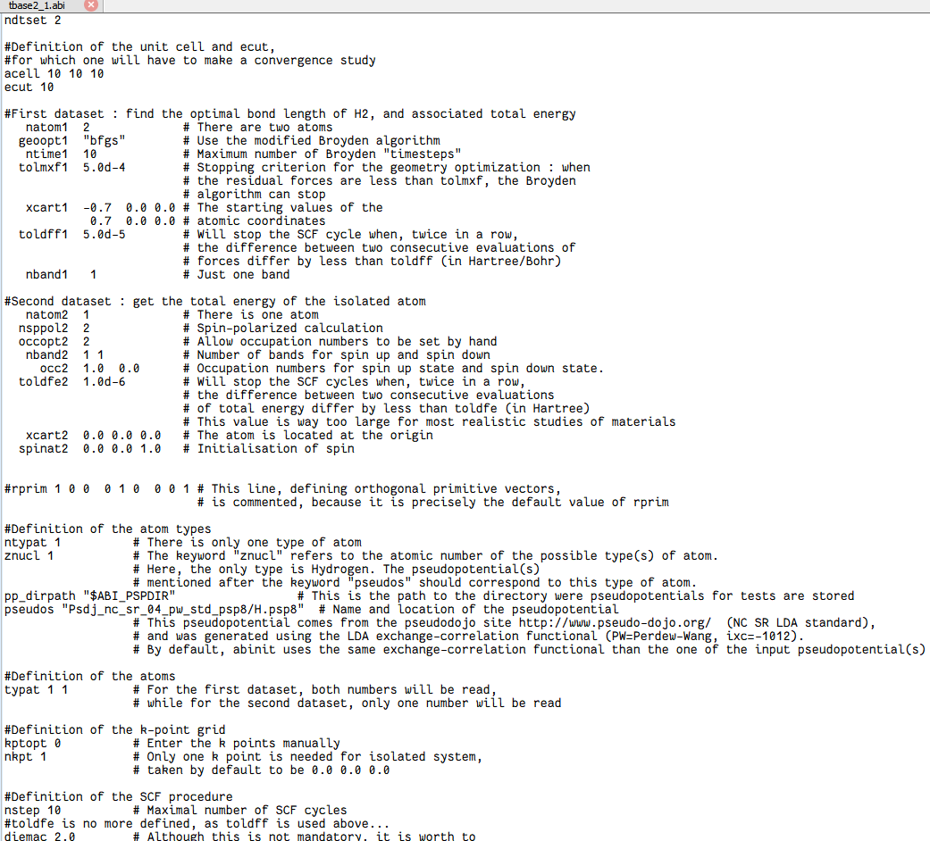
首先打开tbase2_1.abi
核心参数
ndtset 2告诉 ABINIT:下面要连跑 两个dataset,分别是 dataset 1 和 dataset 2。
为区分分段任务,不同dataset的必要参数后面可以加1或2进行区分,而共同参数可不加。
dataset 1:优化 H₂ 几何
natom1 2#dataset 1 里有 2 个原子(H₂)。geoopt1 "bfgs" #用 BFGS 算法做离子弛豫(找能量最低结构)。ntime1 10 #最多允许 10 步离子步。tolmxf1 5.0d-4 #当每个原子受力都小于 5×10⁻⁴ Hartree/Bohr 时就认为优化完成。xcart1 -0.7 0.00.0 #起始坐标(Bohr 为单位):两个 H 原子放在 x 轴上,间距 1.4 Bohr≈0.74 Å,接近实验键长。 0.7 0.00.0toldff1 5.0d-5 #电子自洽(SCF)循环的收敛判据:连续两步力的变化小于 5×10⁻⁵ 就停。nband1 1 #只算 1 条能带(H₂ 分子 σ 成键轨道已占满,导带空着,但这里只放 1 条带足够)。dataset 2:算孤立 H 原子
natom2 1nsppol2 2 #做自旋极化计算(↑↓ 分开)。 occopt2 2 #手工给定 occupation 数。nband2 11 # 自旋向上、向下各放 1 条带。toldfe2 1.0e-6 #能量收敛阈值 10⁻⁶ Hartree。xcart2 0.00.00.0 #给原子一个初始自旋方向(沿 z),帮助程序找到磁解。公用参数保持原有格式
acell 101010ecut 10ntypat 1 # There is only one type of atomznucl 1typat 11 # For the first dataset, both numbers will be read,#Definition of the k-point gridkptopt 0 # Enter the k points manuallynkpt 1 # Only one k point is needed for isolated system,nstep 10 # Maximal number of SCF cyclesdiemac 2.0任务详情:
先让 H₂ 在 10³ Bohr³ 的大盒子里 relax 出最优键长;
再算一个完全自旋极化的孤立 H 原子;
两者总能量差就是 H₂ 的键能(-E_b = E_H₂ – 2×E_H)。
运行ABINIT
abinit tbase2_1.abi >& log2-1 &可以从log文件或者abo文件中查找出实际结构的能量和原子位置
#grep etotal log2-1 etotal1 -1.1182883137E+00 etotal2 -4.7393103688E-01#grep xcart1 log2-1 xcart1 -7.0000000000E-01 0.0000000000E+00 0.0000000000E+00 xcart1 -7.4307169181E-01 0.0000000000E+00 0.0000000000E+00
截断能测试
打开tbase2_2.abi
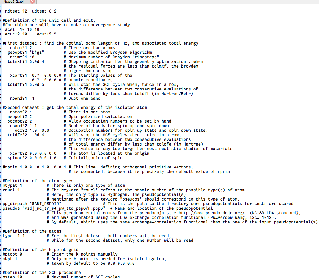
文档里存在很多问号,这个不是格式错误,而是必要的循环标志,类似于for的参数循环。
核心参数
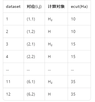
ndtset 12 udtset 62ndtset 12:总共跑 12 个dataset。
udtset 6 2:把 12 个dataset排成 6×2 的二维循环,即
外层循环变量 i 从 1→6,内层循环变量 j 从 1→2,共 6×2=12 组。
在 ABINIT 里用 ? 占位符表示“循环维度”:
?1 代表 j=1 的列(H₂ 分子计算);
?2 代表 j=2 的列(孤立 H 原子计算);
ecut? 代表 i 循环(不同 ecut 值)。
ecut:? 10 ecut+? 5ecut:? 10:对 i=1 的外层循环,起始 ecut = 10 Hartree。
ecut+? 5:每换下一组 i,ecut 递增 5 Hartree。
于是 6 组 ecut 依次为:10, 15, 20, 25, 30, 35 Hartree。
内层 j=1,2 共用同一 ecut(i)。
所有带 ?1 的关键字只对 j=1(H₂ 分子)生效;
所有带 ?2 的关键字只对 j=2(孤立 H 原子)生效;
ABINIT 会自动把 12 个 dataset 拆成:
其余关键字(acell、typat、kptopt、diemac 等)都不带 ?,表示全部 12 个 dataset 共用同一值,不再重复写 12 次。
#First dataset : find the optimal bond length of H2, and associated total energy natom?12 # There are two atoms geoopt?1"bfgs" # Use the modified Broyden algorithm ntime?110 # Maximum number of Broyden "timesteps" tolmxf?15.0d-4 # Stopping criterion for the geometry optimization : when # the residual forces are less than tolmxf, the Broyden # algorithm can stop xcart?1-0.7 0.00.0 # The starting values of the 0.7 0.00.0# atomic coordinates toldff?15.0d-5 # Will stop the SCF cycle when, twice in a row, # the difference between two consecutive evaluations of # forces differ by less than toldff (in Hartree/Bohr) nband?1 1 # Just one band#Second dataset : get the total energy of the isolated atom natom?21 # There is one atom nsppol?22 # Spin-polarized calculation occopt?22 # Allow occupation numbers to be set by hand nband?211 # Number of bands for spin up and spin down occ?21.0 0.0 # Occupation numbers for spin up state and spin down state. toldfe?21.0d-6 # Will stop the SCF cycles when, twice in a row, # the difference between two consecutive evaluations # of total energy differ by less than toldfe (in Hartree) # This value is way too large for most realistic studies of materials xcart?20.00.00.0 # The atom is located at the origin spinat?20.00.01.0 # Initialisation of spin运行ABINIT
abinit tbase2_2.abi >& log2-2 &
可以从log文件或者abo文件中查找出实际结构的能量和原子位置
读出的参数会按着i和j的编号进行排序,比如:
etotal42 就是第一个序列dataset 里第4个,也就是ecut为20的情况下的第二个序列dataset里的孤立H原子的计算。
$ grep etotal log2-2
           etotal11   -1.1182883137E+00           etotal12   -4.7393103688E-01           etotal21   -1.1325211211E+00           etotal22   -4.7860857539E-01           etotal31   -1.1374371581E+00           etotal32   -4.8027186429E-01           etotal41   -1.1389569555E+00           etotal42   -4.8083335144E-01           etotal51   -1.1394234882E+00           etotal52   -4.8101478048E-01           etotal61   -1.1395511942E+00           etotal62   -4.8107063412E-01
$ grep xcart log2-2
xcart11 -7.4307169181E-01 0.0000000000E+00 0.0000000000E+00 xcart12 0.0000000000E+00 0.0000000000E+00 0.0000000000E+00 xcart21 -7.3687974546E-01 0.0000000000E+00 0.0000000000E+00 xcart22 0.0000000000E+00 0.0000000000E+00 0.0000000000E+00 xcart31 -7.3014665027E-01 0.0000000000E+00 0.0000000000E+00 xcart32 0.0000000000E+00 0.0000000000E+00 0.0000000000E+00 xcart41 -7.2642579309E-01 0.0000000000E+00 0.0000000000E+00 xcart42 0.0000000000E+00 0.0000000000E+00 0.0000000000E+00 xcart51 -7.2563260546E-01 0.0000000000E+00 0.0000000000E+00 xcart52 0.0000000000E+00 0.0000000000E+00 0.0000000000E+00 xcart61 -7.2554339763E-01 0.0000000000E+00 0.0000000000E+00 xcart62 0.0000000000E+00 0.0000000000E+00 0.0000000000E+00
分子盒acell 的收敛测试
打开tbase2_3.abi
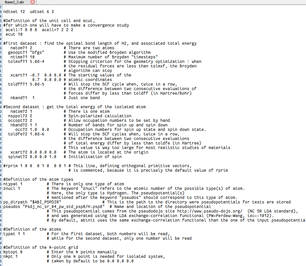
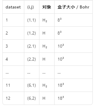
把“外层循环变量”从 ecut 换成了 acell。
acell:? 888 acell+? 222acell:? 8 8 8
对 i = 1 的外层循环,起始盒子边长 8×8×8 Bohr。
acell+? 2 2 2
每进下一组 i,三个边长同时 +2 Bohr。
于是 6 组 acell 依次为:
8³ → 10³ → 12³ → 14³ → 16³ → 18³ Bohr。
内层 j = 1,2 共用同一盒子尺寸。
6 个逐级增大的盒子尺寸自动扫描,快速找到“大盒子极限”。
运行ABINIT
abinit tbase2_3.abi >& log2-3 &可以从log文件或者abo文件中查找出实际结构的能量和原子位置
$ grep etotal log2-3
           etotal11   -1.1305202335E+00           etotal12   -4.8429570903E-01           etotal21   -1.1182883137E+00           etotal22   -4.7393103688E-01           etotal31   -1.1165450484E+00           etotal32   -4.7158917506E-01           etotal41   -1.1165327748E+00           etotal42   -4.7136118536E-01           etotal51   -1.1167740301E+00           etotal52   -4.7128698890E-01           etotal61   -1.1168374331E+00           etotal62   -4.7129589330E-01
$ grep xcart log2-3
xcart11 -7.6471149217E-01 0.0000000000E+00 0.0000000000E+00 xcart12 0.0000000000E+00 0.0000000000E+00 0.0000000000E+00 xcart21 -7.4307169181E-01 0.0000000000E+00 0.0000000000E+00 xcart22 0.0000000000E+00 0.0000000000E+00 0.0000000000E+00 xcart31 -7.3778405090E-01 0.0000000000E+00 0.0000000000E+00 xcart32 0.0000000000E+00 0.0000000000E+00 0.0000000000E+00 xcart41 -7.3794243127E-01 0.0000000000E+00 0.0000000000E+00 xcart42 0.0000000000E+00 0.0000000000E+00 0.0000000000E+00 xcart51 -7.3742475720E-01 0.0000000000E+00 0.0000000000E+00 xcart52 0.0000000000E+00 0.0000000000E+00 0.0000000000E+00 xcart61 -7.3733248368E-01 0.0000000000E+00 0.0000000000E+00 xcart62 0.0000000000E+00 0.0000000000E+00 0.0000000000E+00
tbase2_4.abi和tbase2_5.abi分别为最终收敛参数的计算和泛函的改变,这里不再细说。
因H2分子只需要采用Γ单点计算,后续K点收敛测试便使用Si的计算来说明。
Si的初步自洽计算
打开tbase3_1.abi
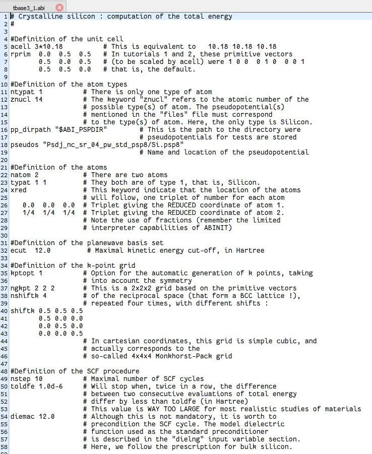
核心参数
acell 3*10.18 #立方 conventional cell 边长 10.18 Bohr(≈ 5.43 Å),#3* 是 ABINIT 的简写,等价于 10.1810.1810.18。rprim 0.0 0.5 0.5 0.5 0.0 0.5 0.5 0.5 0.0 #面心立方 (fcc) 原始矢量(未乘 acell 前)。#这样组合后,实际得到的是 金刚石立方原胞(两个 Si 原子 basis)。ntypat 1znucl 14 #只有一种元素 → 原子序数 14 → Si。pseudos "Psdj_nc_sr_04_pw_std_psp8/Si.psp8"#使用 pseudodojo 标准 LDA-PW 赝势;文件名里的 pw 代表 Perdew-Wang LDA。natom 2typat 11 #原胞里只放 2 个 Si 原子,符合金刚石结构最小原胞。xred#归约坐标(相对原胞矢量): 0.0 0.0 0.0 #原子 1 在 (0,0,0) 1/4 1/4 1/4 #原子 2 在 (1/4 1/4 1/4)ecut 12.0 #平面波截断 12 Ha kptopt 1 #自动对称化生成 k 点ngkpt 222nshiftk 4shiftk 0.50.50.5 0.50.00.0 0.00.50.0 0.00.00.5 #2×2×2 基础网格 + 4 组偏移 → 实际得到 4×4×4 Monkhorst-Pack 网格(64 个 k 点,经对称性折叠后 ≈ 10 个)。nstep 10toldfe 1.0d-6#最多 10 步电子自洽;能量收敛阈值 10⁻⁶ Ha diemac 12.0diemac 12.0运行ABINIT
abinit tbase3_1.abi >& log3-1 &可以从log文件或者abo文件中查找出实际结构的能量和原子位置
$ grep etotal log3-1 etotal -8.5187390642E+00$ grep xcart log3-1
xcart 0.0000000000E+00 0.0000000000E+00 0.0000000000E+00 xcart 0.0000000000E+00 0.0000000000E+00 0.0000000000E+00
tbase3_2.abi 是一个错误例子,展示了写错nkpt参数后产生的情况,这里直接打开tbase3_3.abi
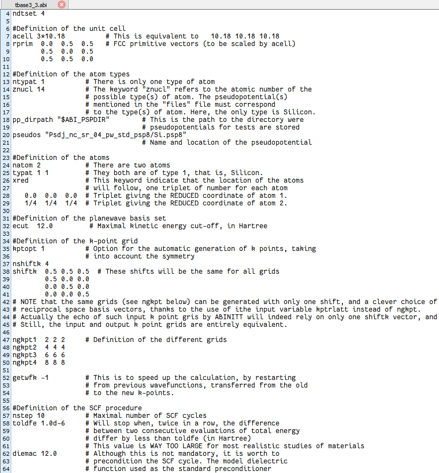
核心参数
ndtset 4 #总共跑 4 个 dataset,对应 4 套 k 网格。ngkpt1 222ngkpt2 444ngkpt3 666ngkpt4 888getwfk -1 #波函数递推加速运行ABINIT
abinit tbase3_3.abi >& log3-3 &
根据输出文件,以下是不同k点网格总能量的演化:
grep etotal log3-3 etotal1 -8.5187390642E+00 etotal2 -8.5250179735E+00 etotal3 -8.5251232908E+00 etotal4 -8.5251270559E+00
