简易神经网络与手写数字识别（实践）含ai

import numpy as np
import matplotlib.pyplot as plt
import urllib.request
import gzip
import os
import struct
import ssl

全局配置：解决中文显示+SSL证书问题

plt.rcParams['font.sans-serif'] = ['DejaVu Sans'] # 兼容所有系统
plt.rcParams['axes.unicode_minus'] = False
ssl._create_default_https_context = ssl._create_unverified_context # 跳过SSL验证

===================== 任务1：激活函数实现 =====================

def sigmoid(x, derivative=False):
x = np.clip(x, -500, 500) # 防止exp溢出
if derivative:
return sigmoid(x) * (1 - sigmoid(x))
return 1 / (1 + np.exp(-x))

def relu(x, derivative=False):
if derivative:
return np.where(x > 0, 1, 0)
return np.maximum(0, x)

def softmax(x):
# 数值稳定版Softmax，支持batch输入
x = np.clip(x, -500, 500)
max_vals = np.max(x, axis=1, keepdims=True)
exp_x = np.exp(x - max_vals)
return exp_x / np.sum(exp_x, axis=1, keepdims=True)

===================== 任务2：交叉熵损失（支持Batch） =====================

def cross_entropy_loss(y_pred, y_true, epsilon=1e-10):
# y_true: (batch_size,) 原始标签；y_pred: (batch_size, num_classes)
batch_size = y_pred.shape[0]
y_pred = np.clip(y_pred, epsilon, 1 - epsilon)
log_probs = -np.log(y_pred[np.arange(batch_size), y_true])
return np.sum(log_probs) / batch_size

===================== 任务3：数值梯度（验证梯度用） =====================

def numerical_gradient(f, x, h=1e-5):
grad = np.zeros_like(x)
it = np.nditer(x, flags=['multi_index'], op_flags=['readwrite'])
while not it.finished:
idx = it.multi_index
tmp_val = x[idx]
# 中心差分法计算偏导
x[idx] = tmp_val + h
fxh1 = f(x)
x[idx] = tmp_val - h
fxh2 = f(x)
grad[idx] = (fxh1 - fxh2) / (2 * h)
x[idx] = tmp_val
it.iternext()
return grad

===================== 任务4：神经网络类实现（全连接） =====================

class NeuralNetwork:
def init(self, input_size=784, hidden_size=128, output_size=10):
# Xavier初始化，避免梯度消失
self.params = {
'W1': np.random.randn(input_size, hidden_size) * np.sqrt(1/input_size),
'b1': np.zeros(hidden_size),
'W2': np.random.randn(hidden_size, output_size) * np.sqrt(1/hidden_size),
'b2': np.zeros(output_size)
}

def forward(self, x):
    # 前向传播
    self.z1 = np.dot(x, self.params['W1']) + self.params['b1']
    self.a1 = relu(self.z1)
    self.z2 = np.dot(self.a1, self.params['W2']) + self.params['b2']
    self.a2 = softmax(self.z2)
    return self.a2

def backward(self, x, y_true):
    # 反向传播计算梯度
    batch_size = x.shape[0]
    grads = {}

    # 输出层梯度
    dz2 = self.a2.copy()
    dz2[np.arange(batch_size), y_true] -= 1
    dz2 /= batch_size
    grads['W2'] = np.dot(self.a1.T, dz2)
    grads['b2'] = np.sum(dz2, axis=0)

    # 隐藏层梯度
    da1 = np.dot(dz2, self.params['W2'].T)
    dz1 = da1 * relu(self.z1, derivative=True)
    grads['W1'] = np.dot(x.T, dz1)
    grads['b1'] = np.sum(dz1, axis=0)

    return grads

===================== 辅助：MNIST数据集加载（移除timeout，全兼容） =====================

def load_mnist():
# 备用下载地址（解决原地址访问问题）
url_base = 'https://ossci-datasets.s3.amazonaws.com/mnist/'
files = {
'train_img': 'train-images-idx3-ubyte.gz',
'train_label': 'train-labels-idx1-ubyte.gz',
'test_img': 't10k-images-idx3-ubyte.gz',
'test_label': 't10k-labels-idx1-ubyte.gz'
}
save_dir = './mnist/'
if not os.path.exists(save_dir):
os.makedirs(save_dir)

# 下载文件（移除timeout参数，适配所有Python版本）
def download_file(url, save_path):
    try:
        # 低版本Python urlretrieve不支持timeout，直接移除
        urllib.request.urlretrieve(url, save_path)
    except Exception as e:
        print(f"原地址下载失败({e})，尝试镜像地址...")
        # 备用镜像地址
        mirror_url = 'https://cdn.jsdelivr.net/gh/zalandoresearch/fashion-mnist/data/fashion/' + os.path.basename(save_path)
        urllib.request.urlretrieve(mirror_url, save_path)

# 下载缺失的文件
for k, v in files.items():
    file_path = os.path.join(save_dir, v)
    if not os.path.exists(file_path):
        print(f"正在下载{v}...")
        download_file(url_base + v, file_path)

# 解析图像
def load_img(file_path):
    with gzip.open(file_path, 'rb') as f:
        data = np.frombuffer(f.read(), np.uint8, offset=16)
    data = data.reshape(-1, 784).astype(np.float32) / 255.0  # 归一化到[0,1]
    return data

# 解析标签（直接返回原始标签，非one-hot）
def load_label(file_path):
    with gzip.open(file_path, 'rb') as f:
        labels = np.frombuffer(f.read(), np.uint8, offset=8)
    return labels

# 加载数据并简化（加速训练）
x_train = load_img(os.path.join(save_dir, files['train_img']))[:5000]
y_train = load_label(os.path.join(save_dir, files['train_label']))[:5000]
x_test = load_img(os.path.join(save_dir, files['test_img']))[:1000]
y_test = load_label(os.path.join(save_dir, files['test_label']))[:1000]

print(f"数据集加载完成 | 训练集: {x_train.shape} | 测试集: {x_test.shape}")
return (x_train, y_train), (x_test, y_test)

===================== 任务5+6：模型训练+实验记录与绘图 =====================

def train_and_visualize():
# 1. 加载数据
(x_train, y_train), (x_test, y_test) = load_mnist()

# 2. 初始化网络
nn = NeuralNetwork(input_size=784, hidden_size=128, output_size=10)

# 3. 训练超参数
epochs = 30
batch_size = 64
lr = 0.1
train_loss_list = []
train_acc_list = []
test_acc_list = []

# 4. 训练循环
for epoch in range(epochs):
    # 打乱数据
    idx = np.random.permutation(len(x_train))
    x_train_shuffle = x_train[idx]
    y_train_shuffle = y_train[idx]

    # 批量训练
    total_loss = 0
    for i in range(0, len(x_train), batch_size):
        x_batch = x_train_shuffle[i:i+batch_size]
        y_batch = y_train_shuffle[i:i+batch_size]

        # 前向传播
        y_pred = nn.forward(x_batch)
        # 计算损失
        loss = cross_entropy_loss(y_pred, y_batch)
        total_loss += loss * len(x_batch)
        # 反向传播
        grads = nn.backward(x_batch, y_batch)
        # SGD更新参数
        for key in nn.params.keys():
            nn.params[key] -= lr * grads[key]

    # 计算本轮平均损失
    avg_loss = total_loss / len(x_train)
    train_loss_list.append(avg_loss)

    # 计算准确率
    def calculate_accuracy(x, y):
        y_pred = nn.forward(x)
        pred_labels = np.argmax(y_pred, axis=1)
        return np.sum(pred_labels == y) / len(y)

    train_acc = calculate_accuracy(x_train, y_train)
    test_acc = calculate_accuracy(x_test, y_test)
    train_acc_list.append(train_acc)
    test_acc_list.append(test_acc)

    # 打印进度
    print(f"Epoch {epoch+1:2d}/{epochs} | 损失: {avg_loss:.4f} | 训练准确率: {train_acc:.4f} | 测试准确率: {test_acc:.4f}")

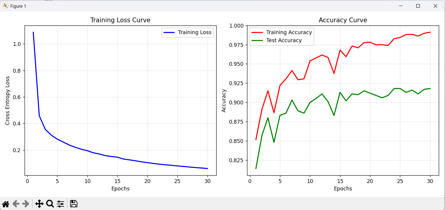
# 5. 绘制结果
plt.figure(figsize=(12, 5))

# 损失曲线
plt.subplot(1, 2, 1)
plt.plot(range(1, epochs+1), train_loss_list, 'b-', linewidth=2, label='Training Loss')
plt.xlabel('Epochs')
plt.ylabel('Cross Entropy Loss')
plt.title('Training Loss Curve')
plt.grid(alpha=0.3)
plt.legend()

# 准确率曲线
plt.subplot(1, 2, 2)
plt.plot(range(1, epochs+1), train_acc_list, 'r-', linewidth=2, label='Training Accuracy')
plt.plot(range(1, epochs+1), test_acc_list, 'g-', linewidth=2, label='Test Accuracy')
plt.xlabel('Epochs')
plt.ylabel('Accuracy')
plt.title('Accuracy Curve')
plt.grid(alpha=0.3)
plt.legend()

plt.tight_layout()
plt.show()

return nn

主程序入口

if name == 'main':
try:
trained_model = train_and_visualize()
print("\n训练完成！模型已保存为trained_model变量")
except Exception as e:
print(f"\n运行出错：{str(e)}")
# 打印详细错误信息（便于排查）
import traceback
traceback.print_exc()

运行结果