迁移学习（DANN）《Unsupervised Domain Adaptation by Backpropagation》

论文信息

论文标题：Domain-Adversarial Training of Neural Networks
论文作者：Yaroslav Ganin, Evgeniya Ustinova, Hana Ajakan, Pascal Germain
论文来源：JMLR 2016
论文地址：download 
论文代码：download
引用次数：5292

1 域适应

　　We consider classification tasks where $X$ is the input space and $Y=\{0,1, \ldots, L-1\}$ is the set of $L$ possible labels. Moreover, we have two different distributions over $X \times Y$ , called the source domain $\mathcal{D}_{\mathrm{S}}$ and the target domain $\mathcal{D}_{\mathrm{T}}$ . An unsupervised domain adaptation learning algorithm is then provided with a labeled source sample $S$ drawn i.i.d. from $\mathcal{D}_{\mathrm{S}}$ , and an unlabeled target sample $T$ drawn i.i.d. from $\mathcal{D}_{\mathrm{T}}^{X}$ , where $\mathcal{D}_{\mathrm{T}}^{X}$ is the marginal distribution of $\mathcal{D}_{\mathrm{T}}$ over $X$ .

　　　　$S=\left\{\left(\mathbf{x}_{i}, y_{i}\right)\right\}_{i=1}^{n} \sim\left(\mathcal{D}_{\mathrm{S}}\right)^{n}$

　　　　$T=\left\{\mathbf{x}_{i}\right\}_{i=n+1}^{N} \sim\left(\mathcal{D}_{\mathrm{T}}^{X}\right)^{n^{\prime}}$

　　with $N=n+n^{\prime}$ being the total number of samples. The goal of the learning algorithm is to build a classifier $\eta: X \rightarrow Y$ with a low target risk

　　　　$R_{\mathcal{D}_{\mathrm{T}}}(\eta)=\operatorname{Pr}_{(\mathbf{x}, y) \sim \mathcal{D}_{\mathrm{T}}}(\eta(\mathbf{x}) \neq y),$

　　while having no information about the labels of $\mathcal{D}_{\mathrm{T}}$ .

2 Domain Divergence

　　假设：如果数据来自源域，域标签为 $1$，如果数据来自目标域，域标签为 $0$。

　　Definition 1. Given two domain distributions  $\mathcal{D}_{\mathrm{S}}^{X}$  and  $\mathcal{D}_{\mathrm{T}}^{X}$  over  $X$ , and a hypothesis class  $\mathcal{H}$ , the  $\mathcal{H}\text{-divergence}$ between  $\mathcal{D}_{\mathrm{S}}^{X}$  and  $\mathcal{D}_{\mathrm{T}}^{X}$  is

　　　　$d_{\mathcal{H}}\left(\mathcal{D}_{\mathrm{S}}^{X}, \mathcal{D}_{\mathrm{T}}^{X}\right)=    2 \;\underset{\eta \in \mathcal{H}}{\text{sup}}\;\left|\operatorname{Pr}_{\mathbf{x} \sim \mathcal{D}_{\mathrm{S}}^{X}}\; [\eta(\mathbf{x})=1]-\operatorname{Pr}_{\mathbf{x} \sim \mathcal{D}_{\mathrm{T}}^{X}}\;[\eta(\mathbf{x})=1]\right|$

　　$\mathcal{H}\text{-divergence}$ 换言之：在假设空间  $\mathcal{H}$  中，找到一个函数 $\mathrm{h}$，使 $\operatorname{Pr}_{x \sim \mathcal{D}}[h(x)=1]$  尽可能大，而 $\operatorname{Pr}_{x \sim \mathcal{D}^{\prime}}[h(x)=1]$ 尽可能小。

　　可通过计算样本 $S \sim\left(\mathcal{D}_{\mathrm{S}}^{X}\right)^{n}$ 和 $T \sim\left(\mathcal{D}_{\mathrm{T}}^{X}\right)^{n^{\prime}}$ 之间的经验 $\text { H-divergence }$ 来近似：

　　　　$\hat{d}_{\mathcal{H}}(S, T)=2\left(1- \underset{\eta \in \mathcal{H}}{\text{min}} \left[\frac{1}{n} \sum\limits_{i=1}^{n} I\left[\eta\left(\mathbf{x}_{i}\right)=0\right]+\frac{1}{n^{\prime}} \sum\limits _{i=n+1}^{N} I\left[\eta\left(\mathbf{x}_{i}\right)=1\right]\right]\right) \quad\quad(1)$

　　其中，$I[a]$ 是指示函数：若 $a$ 为真时，$I[a] = 1$，否则 $I[a] = 0$。

3 Proxy Distance

　　由于经验 $\mathcal{H}\text{-divergence}$ 难以精确计算，可使用判别 源样本与目标样本 的学习算法完成近似。

　　构造新的数据集 $U$ ：

　　　　$U=\left\{\left(\mathbf{x}_{i}, 0\right)\right\}_{i=1}^{n} \cup\left\{\left(\mathbf{x}_{i}, 1\right)\right\}_{i=n+1}^{N}\quad\quad(2)$

　　使用 $\mathcal{H}\text{-divergence}$ 的近似表示 $\text{Proxy A-distance(PAD)}$：

　　　　$\hat{d}_{\mathcal{A}}=2(1-2 \epsilon)\quad\quad(3)$

　　其中，$\epsilon$ 为 源域和目标域样本的分类泛化误差

4 Method

　　假设输入空间由 $m$ 维向量 $X=\mathbb{R}^{m}$ 构成，隐层 $G_{f}: X \rightarrow \mathbb{R}^{D}$ ，由 $  (\mathbf{W}, \mathbf{b}) \in \mathbb{R}^{D \times m} \times \mathbb{R}^{D}  $ 参数化：

　　　　$\begin{array}{l}G_{f}(\mathbf{x} ; \mathbf{W}, \mathbf{b})=\operatorname{sigm}(\mathbf{W} \mathbf{x}+\mathbf{b}) \\\text { with } \operatorname{sigm}(\mathbf{a})=\left[\frac{1}{1+\exp \left(-a_{i}\right)}\right]_{i=1}^{|\mathbf{a}|}\end{array}\quad\quad(4)$

　　预测层 $G_{y}: \mathbb{R}^{D} \rightarrow[0,1]^{L}$，由 $(\mathbf{V}, \mathbf{c}) \in \mathbb{R}^{L \times D} \times \mathbb{R}^{L}$ 参数化：

　　　　$\begin{array}{l}G_{y}\left(G_{f}(\mathbf{x}) ; \mathbf{V}, \mathbf{c}\right)=\operatorname{softmax}\left(\mathbf{V} G_{f}(\mathbf{x})+\mathbf{c}\right)\\\text { with }\quad \operatorname{softmax}(\mathbf{a})=\left[\frac{\exp \left(a_{i}\right)}{\sum_{j=1}^{|a|} \exp \left(a_{j}\right)}\right]_{i=1}^{|\mathbf{a}|}\end{array}$

　　其中 $L=|Y|$。

　　给定一个源样本 $\left(\mathbf{x}_{i}, y_{i}\right)$，使用正确标签的负对数概率：

　　　　$\mathcal{L}_{y}\left(G_{y}\left(G_{f}\left(\mathbf{x}_{i}\right)\right), y_{i}\right)=\log \frac{1}{G_{y}\left(G_{f}(\mathbf{x})\right)_{y_{i}}}$

　　对神经网络的训练会导致源域上的以下优化问题：

　　　　$\underset{\mathbf{W}, \mathbf{b}, \mathbf{V}, \mathbf{c}}{\text{min}} \left[\frac{1}{n} \sum_{i=1}^{n} \mathcal{L}_{y}^{i}(\mathbf{W}, \mathbf{b}, \mathbf{V}, \mathbf{c})+\lambda \cdot R(\mathbf{W}, \mathbf{b})\right]\quad\quad(5)$

　　其中，$\mathcal{L}_{y}^{i}(\mathbf{W}, \mathbf{b}, \mathbf{V}, \mathbf{c})=\mathcal{L}_{y}\left(G_{y}\left(G_{f}\left(\mathbf{x}_{i} ; \mathbf{W}, \mathbf{b}\right) ; \mathbf{V}, \mathbf{c}\right), y_{i}\right)$，$R(\mathbf{W}, \mathbf{b})$ 是一个正则化项。

　　域正则化器引出想法：借用 $\text{Definition 1}$ 的 $\mathcal{H}$-divergence 推导出的域正则化器。

　　源样本、目标样本分别表示为

　　　　$S\left(G_{f}\right)=\left\{G_{f}(\mathbf{x}) \mid \mathbf{x} \in S\right\}$

　　　　$T\left(G_{f}\right)=\left\{G_{f}(\mathbf{x}) \mid \mathbf{x} \in T\right\}$

　　在 $\text{Eq.1}$ 的基础上，给出样本 $S\left(G_{f}\right)$ 和 $T\left(G_{f}\right)$ 之间的经验 $\mathcal{H}\text{-divergence}$：

　　　　$\hat{d}_{\mathcal{H}}\left(S\left(G_{f}\right), T\left(G_{f}\right)\right)=2\left(1-\min _{\eta \in \mathcal{H}}\left[\frac{1}{n} \sum\limits_{i=1}^{n} I\left[\eta\left(G_{f}\left(\mathbf{x}_{i}\right)\right)=0\right]+\frac{1}{n^{\prime}} \sum\limits_{i=n+1}^{N} I\left[\eta\left(G_{f}\left(\mathbf{x}_{i}\right)\right)=1\right]\right]\right) \quad\quad(6)$

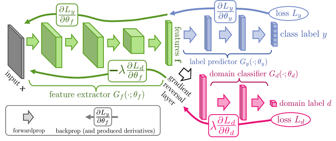
　　域分类器 $G_{d}: \mathbb{R}^{D} \rightarrow[0,1]$ ，由 $(\mathbf{u}, z) \in \mathbb{R}^{D} \times \mathbb{R}$ 参数化，计算了输入来自源域 $\mathcal{D}_{\mathrm{S}}^{X}$ 或目标域 $\mathcal{D}_{\mathrm{T}}^{X}$ 的概率：

　　　　$G_{d}\left(G_{f}(\mathbf{x}) ; \mathbf{u}, z\right)=\operatorname{sigm}\left(\mathbf{u}^{\top} G_{f}(\mathbf{x})+z\right)\quad\quad(7)$

　　因此，域分类器的交叉熵损失如下：

　　　　$\mathcal{L}_{d}\left(G_{d}\left(G_{f}\left(\mathbf{x}_{i}\right)\right), d_{i}\right)=d_{i} \log \frac{1}{G_{d}\left(G_{f}\left(\mathbf{x}_{i}\right)\right)}+\left(1-d_{i}\right) \log \frac{1}{1-G_{d}\left(G_{f}\left(\mathbf{x}_{i}\right)\right)}$

　　其中，$d_{i}$ 表示第 $i$ 个样本的二分类域标签。

　　$\text{Eq.5}$ 的目标中添加域自适应项，并给出以下正则化器：

　　　　$R(\mathbf{W}, \mathbf{b})=\underset{\mathbf{u}, z}{\text{max}}  {}\left[-\frac{1}{n} \sum\limits _{i=1}^{n} \mathcal{L}_{d}^{i}(\mathbf{W}, \mathbf{b}, \mathbf{u}, z)-\frac{1}{n^{\prime}} \sum\limits_{i=n+1}^{N} \mathcal{L}_{d}^{i}(\mathbf{W}, \mathbf{b}, \mathbf{u}, z)\right]\quad\quad(8)$

　　其中，$\mathcal{L}_{d}^{i}(\mathbf{W}, \mathbf{b}, \mathbf{u}, z)=\mathcal{L}_{d}\left(G_{d}\left(G_{f}\left(\mathbf{x}_{i} ; \mathbf{W}, \mathbf{b}\right) ; \mathbf{u}, z\right), d_{i}\right)$ 。

　　△：$R(\mathbf{W}, \mathbf{b})$ 试图近似 $\text{Eq.6}$ 的 $\mathcal{H}\text{-divergence}$，因为 $2(1-R(\mathbf{W}, \mathbf{b}))$ 是 $\hat{d}_{\mathcal{H}}\left(S\left(G_{f}\right), T\left(G_{f}\right)\right)$ 的一个替代品。

　　$\text{Eq.5}$ 的完整优化目标重写如下：

　　　　$\begin{array}{l}E(\mathbf{W}, \mathbf{V}, \mathbf{b}, \mathbf{c}, \mathbf{u}, z) \\\quad=\frac{1}{n} \sum\limits _{i=1}^{n} \mathcal{L}_{y}^{i}(\mathbf{W}, \mathbf{b}, \mathbf{V}, \mathbf{c})-\lambda\left(\frac{1}{n} \sum\limits_{i=1}^{n} \mathcal{L}_{d}^{i}(\mathbf{W}, \mathbf{b}, \mathbf{u}, z)+\frac{1}{n^{\prime}} \sum_{i=n+1}^{N} \mathcal{L}_{d}^{i}(\mathbf{W}, \mathbf{b}, \mathbf{u}, z)\right)\end{array}\quad\quad(9)$

　　对应的参数优化 $\hat{\mathbf{W}}$, $\hat{\mathbf{V}}$, $\hat{\mathbf{b}}$, $\hat{\mathbf{c}}$, $\hat{\mathbf{u}}$, $\hat{z}$：

　　　　$\begin{array}{l}(\hat{\mathbf{W}}, \hat{\mathbf{V}}, \hat{\mathbf{b}}, \hat{\mathbf{c}}) & =&  \underset{\mathbf{W}, \mathbf{V}, \mathbf{b}, \mathbf{c}}{\operatorname{arg min}} E(\mathbf{W}, \mathbf{V}, \mathbf{b}, \mathbf{c}, \hat{\mathbf{u}}, \hat{z}) \\(\hat{\mathbf{u}}, \hat{z}) & =&\underset{\mathbf{u}, z}{\operatorname{arg max}} E(\hat{\mathbf{W}}, \hat{\mathbf{V}}, \hat{\mathbf{b}}, \hat{\mathbf{c}}, \mathbf{u}, z)\end{array}$

Generalization to Arbitrary Architectures

　　分类损失和域分类损失：

　　　　$\begin{aligned}\mathcal{L}_{y}^{i}\left(\theta_{f}, \theta_{y}\right) & =\mathcal{L}_{y}\left(G_{y}\left(G_{f}\left(\mathbf{x}_{i} ; \theta_{f}\right) ; \theta_{y}\right), y_{i}\right) \\\mathcal{L}_{d}^{i}\left(\theta_{f}, \theta_{d}\right) & =\mathcal{L}_{d}\left(G_{d}\left(G_{f}\left(\mathbf{x}_{i} ; \theta_{f}\right) ; \theta_{d}\right), d_{i}\right)\end{aligned}$

　　优化目标：

　　　　$E\left(\theta_{f}, \theta_{y}, \theta_{d}\right)=\frac{1}{n} \sum\limits_{i=1}^{n} \mathcal{L}_{y}^{i}\left(\theta_{f}, \theta_{y}\right)-\lambda\left(\frac{1}{n} \sum\limits_{i=1}^{n} \mathcal{L}_{d}^{i}\left(\theta_{f}, \theta_{d}\right)+\frac{1}{n^{\prime}} \sum\limits_{i=n+1}^{N} \mathcal{L}_{d}^{i}\left(\theta_{f}, \theta_{d}\right)\right)  \quad\quad(10)$

　　对应的参数优化 $\hat{\theta}_{f}$, $\hat{\theta}_{y}$, $\hat{\theta}_{d}$：

　　　　$\begin{array}{l}\left(\hat{\theta}_{f}, \hat{\theta}_{y}\right) & =&\underset{\theta_{f}, \theta_{y}}{\operatorname{argmin}} E\left(\theta_{f}, \theta_{y}, \hat{\theta}_{d}\right) \quad\quad(11) \\\hat{\theta}_{d} & =&\underset{\theta_{d}}{\operatorname{argmax}} E\left(\hat{\theta}_{f}, \hat{\theta}_{y}, \theta_{d}\right)\quad\quad(12)\end{array}$

　　 如前所述，由 $\text{Eq.11-Eq.12}$ 定义的鞍点可以作为以下梯度更新的平稳点找到：

　　　　$\begin{array}{l}\theta_{f} \longleftarrow \theta_{f}-\mu\left(\frac{\partial \mathcal{L}_{y}^{i}}{\partial \theta_{f}}-\lambda \frac{\partial \mathcal{L}_{d}^{i}}{\partial \theta_{f}}\right)\quad\quad(13) \\\theta_{y} \longleftarrow \quad \theta_{y}-\mu \frac{\partial \mathcal{L}_{y}^{i}}{\partial \theta_{y}}\quad\quad\quad\quad \quad\quad(14)  \\\theta_{d} \quad \longleftarrow \quad \theta_{d}-\mu \lambda \frac{\partial \mathcal{L}_{d}^{i}}{\partial \theta_{d}}\quad\quad\quad\quad(15)  \\\end{array}$

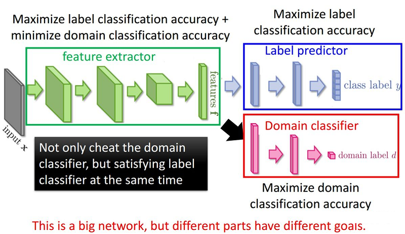
　　整体框架：

　　

---

　　　

 

5 总结

　　问题：

• • 存在梯度消失的问题；
  • 训练过程不稳定；

 

for epoch in range(n_epoch):
    len_dataloader = min(len(dataloader_source), len(dataloader_target))
    data_source_iter = iter(dataloader_source)
    data_target_iter = iter(dataloader_target)

    i = 0
    while i < len_dataloader:
        p = float(i + epoch * len_dataloader) / n_epoch / len_dataloader
        alpha = 2. / (1. + np.exp(-10 * p)) - 1

        # training model using source data
        data_source = data_source_iter.next()
        s_img, s_label = data_source

        class_output, domain_output = my_net(input_data=s_img, alpha=alpha)
        err_s_label = loss_class(class_output, class_label)
        err_s_domain = loss_domain(domain_output, domain_label)

        # training model using target data
        t_img, _ = data_target_iter.next()
        domain_label = torch.ones(batch_size)
        domain_label = domain_label.long()
        _, domain_output = my_net(input_data=t_img, alpha=alpha)
        err_t_domain = loss_domain(domain_output, domain_label)
        err = err_t_domain + err_s_domain + err_s_label

        err.backward()
        optimizer.step()
        i += 1

def forward(self, input_data, alpha):
    feature = self.feature(input_data)
    class_output = self.class_classifier(feature)

    reverse_feature = ReverseLayerF.apply(feature, alpha)
    domain_output = self.domain_classifier(reverse_feature)
    return class_output, domain_output