论文解读（VGAE）《Variational Graph Auto-Encoders》

论文信息

论文标题：Variational Graph Auto-Encoders
论文作者：Thomas Kipf, M. Welling
论文来源：2016, ArXiv
论文地址：download 
论文代码：download 

1 Introduce

　　变分自编码器在图上的应用，该框架可以自行参考变分自编码器。

2 Method

　　变分图自编码器（VGAE ），整体框架如下：

　　

　　

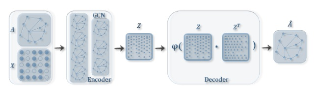
　　框架组成部分：

• • 一个 GCN Encoder
  • 一个简单的内积 Decoder

2.1 Encoder

　　Inference model：一个两层的 GCN 推理模型

　　Step1：获得均值 $\mu$ 和方差的对数 $\log \boldsymbol{\sigma}$

　　　　$\boldsymbol{\mu}=\operatorname{GCN}_{\boldsymbol{\mu}}(\mathbf{X}, \mathbf{A})$

　　　　$\log \boldsymbol{\sigma}=\mathrm{GCN}_{\boldsymbol{\sigma}}(\mathbf{X}, \mathbf{A})$

　　$\log \boldsymbol{\sigma}$ 可正可负，而 $\sigma$ 为正数。

def encode(self, x, adj):
    hidden1 = self.gc1(x, adj)
    return self.gc2(hidden1, adj), self.gc3(hidden1, adj)    

mu, logvar = self.encode(x, adj)

　　注意：这里的GCN 第一层共用，第二层GCN分别输出 $\text{mu}$，$\text{log} \sigma$ 矩阵。

　　Step2：根据均值 $\mu$ 和方差的对数 $\log \boldsymbol{\sigma}$ 获得隐表示 $z$ 

 　　　　$q(\mathbf{Z} \mid \mathbf{X}, \mathbf{A})=\prod_{i=1}^{N} q\left(\mathbf{z}_{i} \mid \mathbf{X}, \mathbf{A}\right) \text { with } \quad q\left(\mathbf{z}_{i} \mid \mathbf{X}, \mathbf{A}\right)=\mathcal{N}\left(\mathbf{z}_{i} \mid \boldsymbol{\mu}_{i}, \operatorname{diag}\left(\boldsymbol{\sigma}_{i}^{2}\right)\right)$

def reparameterize(self, mu, logvar):
    if self.training:
        std = torch.exp(logvar)
        eps = torch.randn_like(std)
        return eps.mul(std).add_(mu)
    else:
        return mu

z = self.reparameterize(mu, logvar)

　　PS：显然 $z$ 的获取是方差 $\text{std}$ 和 正态分布生成的矩阵 $\text{eps}$ 先做哈达玛积，然后在加均值 $\mu$ 。

2.2 Decoder

　　Generative model：根据潜在变量 $z$ 之间的内积给出邻接矩阵 $A$：

　　　　$p(\mathbf{A} \mid \mathbf{Z})=\prod_{i=1}^{N} \prod_{j=1}^{N} p\left(A_{i j} \mid \mathbf{z}_{i}, \mathbf{z}_{j}\right) \text { with } p\left(A_{i j}=1 \mid \mathbf{z}_{i}, \mathbf{z}_{j}\right)=\sigma\left(\mathbf{z}_{i}^{\top} \mathbf{z}_{j}\right)$

　　其中：

• • $\mathbf{A}$ 是邻接矩阵 　　
  • $\sigma(\cdot)$ 是 logistic sigmoid function.　　

class InnerProductDecoder(nn.Module):
    """Decoder for using inner product for prediction."""

    def __init__(self, dropout, act=torch.sigmoid):
        super(InnerProductDecoder, self).__init__()
        self.dropout = dropout
        self.act = act

    def forward(self, z):
        z = F.dropout(z, self.dropout, training=self.training)
        adj = self.act(torch.mm(z, z.t()))
        return adj

self.dc = InnerProductDecoder(dropout, act=lambda x: x)

adj = self.dc(z)

　　PS：计算表示向量 $Z$ 和重建的邻接矩阵 $\hat{\mathbf{A}}$

　　　　$\hat{\mathbf{A}}=\sigma\left(\mathbf{Z Z}^{\top}\right), \text { with } \quad \mathbf{Z}=\operatorname{GCN}(\mathbf{X}, \mathbf{A})$

2.3 Loss function

　　Learning：优化变分下界 $\mathcal{L}$ 的参数 $W_i$ ：

　　这里希望重构出的图（邻接矩阵）和原始的图尽可能相似，当然，由于我们对于latent representation的形式做了一定的假设，同样希望分布与假设中的标准高斯尽可能相似。因此损失函数需要包括两个部分：

　　　　$\mathcal{L}=\mathbb{E}_{q(\mathbf{Z} \mid \mathbf{X}, \mathbf{A})}[\log p(\mathbf{A} \mid \mathbf{Z})]-\mathrm{KL}[q(\mathbf{Z} \mid \mathbf{X}, \mathbf{A}) \| p(\mathbf{Z})]$

　　其中：

• $\operatorname{KL}[q(\cdot) \| p(\cdot)]$ 代表着 $q(\cdot)$  和  $p(\cdot)$ 之间的 KL散度。　　
• 高斯先验 $p(\mathbf{Z})=\prod_{i} p\left(\mathbf{z}_{\mathbf{i}}\right)=\prod_{i} \mathcal{N}\left(\mathbf{z}_{i} \mid 0, \mathbf{I}\right)$　　

　　

 

　　PS：这里的交叉熵是二分类带 sigmoid 且带权的交叉熵。（preds = z , labels = A）

　　权：pos_weight = float(adj.shape[0] * adj.shape[0] - adj.sum()) / adj.sum()   即邻接矩阵中 0 的个数除 1 的个数比。

　　比值：norm = adj.shape[0] * adj.shape[0] / float((adj.shape[0] * adj.shape[0] - adj.sum()) * 2)

def loss_function(preds, labels, mu, logvar, n_nodes, norm, pos_weight):
    cost = norm * F.binary_cross_entropy_with_logits(preds, labels, pos_weight=pos_weight)
    KLD = -0.5 / n_nodes * torch.mean(torch.sum(
        1 + 2 * logvar - mu.pow(2) - logvar.exp().pow(2), 1))
    return cost + KLD

3 Experiment

　　引文网络中链接预测（link prediction）任务的结果如 Table 1 所示。

　　

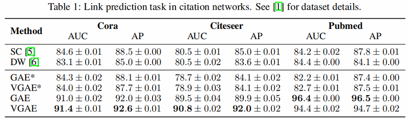
　　GAE* and VGAE* denote experiments without using input features, GAE and VGAE use input features.

4 Other

　　这里 GCN 定义为：
　　　　$\operatorname{GCN}(\mathbf{X}, \mathbf{A})=\tilde{\mathbf{A}} \operatorname{ReLU}\left(\tilde{\mathbf{A}} \mathbf{X} \mathbf{W}_{0}\right) \mathbf{W}_{1}$

　　其中：

• • $\mathbf{W}_{i}$ 代表着权重矩阵　　
  • $\operatorname{GCN}_{\boldsymbol{\mu}}(\mathbf{X}, \mathbf{A})$ 和 $\mathrm{GCN}_{\boldsymbol{\sigma}}(\mathbf{X}, \mathbf{A})$ 共享第一层的权重矩阵 $\mathbf{W}_{0} $
  • $\operatorname{ReLU}(\cdot)=\max (0, \cdot)$　　
  • $\tilde{\mathbf{A}}=\mathbf{D}^{-\frac{1}{2}} \mathbf{A} \mathbf{D}^{-\frac{1}{2}}$ 代表着  symmetrically normalized adjacency matrix　　

import torch
import torch.nn.functional as F
from torch.nn.modules.module import Module
from torch.nn.parameter import Parameter

class GraphConvolution(Module):
    def __init__(self, in_features, out_features, dropout=0., act=F.relu):
        super(GraphConvolution, self).__init__()
        self.in_features = in_features
        self.out_features = out_features
        self.dropout = dropout
        self.act = act
        self.weight = Parameter(torch.FloatTensor(in_features, out_features))
        self.reset_parameters()

    def reset_parameters(self):
        torch.nn.init.xavier_uniform_(self.weight)

    def forward(self, input, adj):
        input = F.dropout(input, self.dropout, self.training)
        support = torch.mm(input, self.weight)
        output = torch.spmm(adj, support)
        output = self.act(output)
        return output

修改历史

2021-03-23 创建文章

2022-06-10 修订文章

2022-06-28 修订文章中的损失函数图片

论文解读目录