论文解读《Cauchy Graph Embedding》

Paper Information

Title：Cauchy Graph Embedding
Authors：Dijun Luo, C. Ding, F. Nie, Heng Huang
Sources：2011, ICML
Others：71 Citations, 30 References

---

Abstract

　　拉普拉斯嵌入（ Laplacian embedding）为图的节点提供了一种低维表示，其中边权值表示节点对象之间的成对相似性。通常假设拉普拉斯嵌入结果保留了低维投影子空间上原始数据的局部拓扑结构，即对于任何一对相似性较大的图节点，它们都应该紧密地嵌入在嵌入空间中。然而，在本文中，我们将证明 Laplacian embedding 往往不能像我们预期的那样很好地保持局部拓扑。为了增强图嵌入中的局部拓扑保持性，我们提出了一种新的 Cauchy Graph Embedding 方法，它通过一个新的目标来保持嵌入空间中原始数据的相似性关系。

1 Introduction

　　从数据嵌入的角度来看，我们可以将无监督嵌入方法分为两类。第一类方法是通过线性变换将数据嵌入到线性空间中，如主成分分析(PCA)(Jolliffe，2002)和多维尺度分析(MDS)(Cox&Cox，2001)。主成分分析和 MDS 都是特征向量方法，可以在高维数据中的线性变量。它们早已广为人知，并被广泛应用于许多机器学习应用程序中。

　　然而，真实数据的底层结构往往是高度非线性的，因此不能用线性流形精确地近似。第二类方法基于不同的目的以非线性的方式嵌入数据。最近提出了几种有前途的非线性方法，包括  IsoMAP (Tenenbaum et al., 2000), Local Linear Embedding (LLE) (Roweis & Saul, 2000), Local Tangent Space Alignment (Zhang & Zha, 2004), Laplacian Embedding/Eigenmap (Hall, 1971; Belkin & Niyogi, 2003; Luo et al., 2009), and Local Spline Embedding (Xiang et al., 2009) etc。通常，他们建立了一个由邻域图导出的二次目标，并求解它的主要特征向量：Isomap 取与最大特征值相关的特征向量；LLE 和 拉普拉斯嵌入 使用与最小特征值相关的特征向量。Isomap 试图保持沿低维流形测量的输入数据的全局成对距离；LLE和拉普拉斯嵌入试图保持数据的局部几何关系。

2 Laplacian Embedding

　　首先介绍 Laplacian embedding 。输入数据是 $n$ 个数据对象之间成对相似性的矩阵 $W$。把 $W$ 看作是一个有 $n$ 个节点的图上的边的权值。其任务是将图中的节点嵌入到具有坐标 $\left(x_{1}, \cdots, x_{n}\right)$ 的一维空间中。目标是，如果 $i$，$j$ 相似(即 $w_{ij}$ 很大)，它们应该在嵌入空间中应该相邻，即 ${(x_i−x_j)}^2$ 应该很小。这可以通过最小化来实现。

　　$\underset{\mathbf{x}}{\text{min}}J(\mathbf{x})=\sum\limits_{i j}\left(x_{i}-x_{j}\right)^{2} w_{i j}\quad\quad\quad(1)$

　　如果最小化 $ \sum\limits_{i j}\left(x_{i}-x_{j}\right)^{2} w_{i j} $ 没有限制，那么可以使得向量 $\mathbf{x} $ 全为 $0$ 向量，这显然不行， 因此加入限制 $\sum\limits_{i} x_{i}^{2}=1$ 。另一个问题是原目标函数具有平移不变性，即将 $x_{i} $ 替换为 $x_{i}+a$ 解不变，这显然不行，所以加入限制 $\sum\limits x_{i}=0$，即 $x$ 围绕在 $0$ 附近。此时原目标函数变为：

　　　　$\begin{array}{c} \min _{\mathbf{x}} \sum\limits_{i j}\left(x_{i}-x_{j}\right)^{2} w_{i j},\\\ \text { s.t. } \sum\limits_{i} x_{i}^{2}=1, \sum\limits_{i} x_{i}=0\end{array}$

　　这个嵌入问题的解决方案很容易得到，因为

　　　　$J(\mathbf{x})=2 \sum\limits_{i j} x_{i}(D-W)_{i j} x_{j}=2 \mathbf{x}^{T}(D-W) \mathbf{x}$

　　其中 $D=\operatorname{diag}\left(d_{1}, \cdots, d_{n}\right)$，$d_{i}=\sum\limits_{j} W_{i j}$。矩阵 $(D-W)$  称为图拉普拉斯算子，最小化嵌入目标的嵌入解由

　　　　$(D-W) \mathbf{x}=\lambda \mathbf{x} \quad \quad \quad (4)$

　　拉普拉斯嵌入在机器学习中得到了广泛的应用，用于保留局部拓扑的图节点的正则化

3 The Local Topology Preserving Property of Graph Embedding

　　本文研究了图嵌入的局部拓扑保持性质。首先给出了局部拓扑保留的定义，并证明了与被广泛接受的概念相反，拉普拉斯嵌入可能不能在嵌入空间中保留原始数据的局部拓扑。

3.1 Local Topology Preserving

　　首先给出了局部拓扑保留的定义。给定一个边权值为 $W=\left(w_{i j}\right) $ 的对称（无向）图，并且对图的 $n$ 个节点具有相应的嵌入 $\left(\mathbf{x}_{1}, \cdots, \mathbf{x}_{n}\right)$。如果以下条件成立，我们假设嵌入保持了局部拓扑

　　　　$\text { if } w_{i j} \geq w_{p q} \text {, then }\left(x_{i}-x_{j}\right)^{2} \leq\left(x_{p}-x_{q}\right)^{2}, \forall i, j, p, q \text {. }\quad\quad \quad (5) $

　　粗略地说，这个定义说，对于任何一对节点 $(i，j)$，它们越相似(边的权重 $w_{ij} $越大)，它们应该嵌入在一起就越近( $|x_i−x_j|$ 应该越小)。

　　拉普拉斯嵌入在机器学习中被广泛应用于保留局部拓扑的概念。作为本文的一个贡献，我们在这里指出这种关于局部拓扑保留的感知概念在许多情况下实际上是错误的。

　　我们的发现有两个方面。首先，在大距离（相似度小）：

　　The quadratic function of the Laplacian embedding emphasizes the large distance pairs, which enforces node pair $(i，j)$ with small $w_{ij}$ to be separated far-away.

　　第二，在小距离（大相似性）处：

　　 The quadratic function of the Laplacian embedding de-emphasizes the small distance pairs, leading to many violations of local topology preserving at small distance pairs.

　　在下面，我们将展示一些示例来支持我们的发现。这一发现的一个结果是，k个最近邻(kNN)类型的分类方法将表现得很差，因为它们依赖于局部拓扑属性。在此基础上，我们提出了一种新的图嵌入方法，它强调小距离（大相似性）数据对，从而强制在嵌入空间中保持局部拓扑。

3.2. Experimental Evidences

　　在  “manifold” data 上，证明了本文提出的方法好于LE。

 　　这里

　　　　$w_{i j}=\exp \left(-\left\|x_{i}-x_{j}\right\|^{2} / \vec{d}^{2}\right)$

　　　　$\bar{d}=\left(\sum\limits _{i \neq j}\left\|x_{i}-x_{j}\right\|\right) /(n(n-1))$

4. Cauchy Embedding

　　在本文中，我们提出了一种新的强调短距离的图嵌入方法，并确保在局部，两个节点越相似，它们在嵌入空间中就越近。

　　我们的方法如下。关键思想是，对于具有大 $ w_{i j}$ 的一对 $(i，j)$，$\left(x_{i}-x_{j}\right)^{2}$ 应该很小，从而使目标函数最小化。现在，如果 $\left(x_{i}-x_{j}\right)^{2} \equiv   \Gamma_{1}\left(\left|x_{i}-x_{j}\right|\right) $ 很小，比如：

　　　　$\frac{\left(x_{i}-x_{j}\right)^{2}}{\left(x_{i}-x_{j}\right)^{2}+\sigma^{2}} \equiv \Gamma_{2}\left(\left|x_{i}-x_{j}\right|\right)$

　　此外，函数 $\Gamma_{1}(\cdot)$ 是单调的，函数 $\Gamma_{2}(\cdot)$ 也是单调的。因此，我们最小化

　　　　$\begin{array}{ll}\underset{\mathbf{x}}{\text{min}} \quad & \sum\limits _{i j} \frac{\left(x_{i}-x_{j}\right)^{2}}{\left(x_{i}-x_{j}\right)^{2}+\sigma^{2}} w_{i j} \\\text { s.t., } & \|\mathbf{x}\|^{2}=1, \mathbf{e}^{T} \mathbf{x}=0 \end{array}$

　　由于

　　　　$\frac{\left(x_{i}-x_{j}\right)^{2}}{\left(x_{i}-x_{j}\right)^{2}+\sigma^{2}}=1-\frac{\sigma^{2}}{\left(x_{i}-x_{j}\right)^{2}+\sigma^{2}}$

　　因此可以简化为 

　　　　$\begin{aligned}\underset{\mathbf{x}}{\text{max}} & \sum_{i j} \frac{w_{i j}}{\left(x_{i}-x_{j}\right)^{2}+\sigma^{2}}, \\\text { s.t. } & \sum_{i} x_{i}^{2}=1, \sum_{i} x_{i}=0 .\end{aligned}$

　　柯西嵌入的目标函数之间的最重要的区别 [ Eq. (6) Eq. (7) ] 与拉普拉斯嵌入的目标函数 [ Eq. (1) ]如下。对于拉普拉斯嵌入，大距离 $\left(x_{i}-\right.   \left.x_{j}\right)^{2}$ 项由于二次形式而贡献更大，而对于柯西嵌入，小距离 $\left(x_{i}-\right.   \left.x_{j}\right)^{2}$ 项贡献更大。这一关键的差异确保了柯西嵌入表现出更强的局部拓扑保持性。

4.1. Multi-dimensional Cauchy Embedding

　　为了表示的简单和清晰，我们首先考虑二维嵌入。对于二维嵌入，每个节点 $i$ 都嵌入在具有坐标 $(x_i，y_i)$ 的二维空间中。通常的拉普拉斯式嵌入可以表示为

　　　　$\begin{array}{ll}\underset{\mathbf{x,y}}{\text{max}} & \sum\limits _{i j}\left[\left(x_{i}-x_{j}\right)^{2}+\left(y_{i}-y_{j}\right)^{2}\right] w_{i j} \quad\quad\quad(8) \\\text { s.t. } & \|\mathbf{x}\|^{2}=1, \mathbf{e}^{T} \mathbf{x}=0 \quad\quad\quad\quad\quad\quad\quad\quad(9)\\& \|\mathbf{y}\|^{2}=1, \mathbf{e}^{T} \mathbf{y}=0 \quad\quad\quad\quad\quad\quad\quad\quad(10)\\& \mathbf{x}^{T} \mathbf{y}=0 \quad\quad\quad\quad\quad\quad\quad\quad\quad\quad\quad\quad(11)\end{array}$

　　其中 $\mathbf{e}=(1, \cdots, 1)^{T}$ . 约束 $\mathbf{x}^{T} \mathbf{y}=0$  很重要，因为没有它，优化得到的最优值为 $\mathbf{x}=\mathbf{y}$。

　　二维柯西矩阵的动机是通过以下优化得到的

　　　　$   \underset{\mathbf{x,y}}{\text{min}} \sum_{i j} \frac{\left(x_{i}-x_{j}\right)^{2}+\left(y_{i}-y_{j}\right)^{2}}{\left(x_{i}-x_{j}\right)^{2}+\left(y_{i}-y_{j}\right)^{2}+\sigma^{2}} w_{i j}\quad\quad\quad (12)$

　　具有相同的约束方程式。(8-11).这将被简化为

　　　　$\underset{\mathbf{x,y}}{\text{min}}\frac{w_{i j}}{\left(x_{i}-x_{j}\right)^{2}+\left(y_{i}-y_{j}\right)^{2}+\sigma^{2}}$

　　一般来说，$p$ 维柯西嵌入到 $R=   \left(\mathbf{r}_{1}, \cdots, \mathbf{r}_{n}\right) \in \Re^{p \times n}$ 是通过优化获得

　　　　$\begin{array}{rl}\underset{\mathbf{R}}{\text{max}} & J(R)=\sum\limits _{i j} \frac{w_{i j}}{\left\|\mathbf{r}_{i}-\mathbf{r}_{j}\right\|^{2}+\sigma^{2}} \quad\quad(14)\\\text { s.t. } & R R^{T}=I, R \mathbf{e}=\mathbf{0}\quad\quad(15)\end{array}$

4.2. Exponential and Gaussian Embedding

　　 In Cauchy embedding the short distance pairs are emphasized more than large distance pairs, in comparison to Laplacian embedding. We can further emphasize the short distance pairs and de-emphasize large distance pairs by the following Gaussian embedding:

　　　　$\begin{array}{r}\underset{\mathbf{x}}{\text{max}} \sum\limits _{i j} \exp \left[-\frac{\left(x_{i}-x_{j}\right)^{2}}{\sigma^{2}}\right] w_{i j}\quad\quad(16) \\\text { s.t., }\|\mathbf{x}\|^{2}=1, \mathbf{e}^{T} \mathbf{x}=0\quad\quad(17) \end{array}$

　　或者指数嵌入

　　　　$\begin{array}{r}\underset{\mathbf{x}}{\text{max}} \sum\limits _{i j} \exp \left[-\frac{\left|x_{i}-x_{j}\right|}{\sigma}\right] w_{i j} \\\text { s.t., }\|\mathbf{x}\|^{2}=1, \mathbf{e}^{T} \mathbf{x}=0\end{array}$

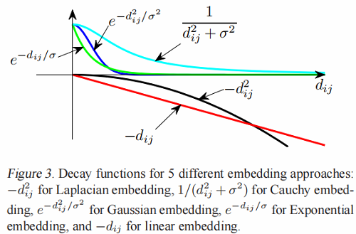
　　一般情况下，我们可以引入 decay function $\Gamma\left(d_{i j}\right)$，并将这三个嵌入目标写为

　　　　$\underset{\mathbf{x}}{\text{max}} \sum\limits _{i j} \Gamma\left(\left|x_{i}-x_{j}\right|\right) w_{i j}, \text { s.t. },\|\mathbf{x}\|^{2}=1, \mathbf{e}^{T} \mathbf{x}=0\quad\quad(20)$

　　下面是一系列的decay functions:

　　　　Laplacian embed: $\quad \Gamma_{\text {Laplace }}\left(d_{i j}\right)=-d_{i j}^{2}\quad\quad(21) $
　　　　Cauchy embed: $\quad \Gamma_{\text {Cauchy }}\left(d_{i j}\right)=\frac{1}{d_{i j}^{2}+\sigma^{2}}\quad\quad(22) $
　　　　Gaussian embed: $\quad \Gamma_{\text {Gaussian }}\left(d_{i j}\right)=e^{-d_{i j}^{2} / \sigma^{2}}\quad\quad(23)$
　　　　Exponential embed: $\quad \Gamma_{\exp }\left(d_{i j}\right)=e^{-d_{i j} / \sigma}\quad\quad(24)$
　　　　Linear embed: $\quad \Gamma_{\text {linear }}\left(d_{i j}\right)=-d_{i j} \quad\quad(25)$

　　我们讨论了衰变函数的两个性质。

• • 对衰减函数有一个要求：$\Gamma(d)$ 必须是随着 $d$ 的增加而单调递减的。如果违反了这种单调性，那么嵌入就没有意义了。　　
  • 衰减函数在一个常数之前是未定义的，即 $\Gamma^{\prime}\left(d_{i j}\right)=\Gamma\left(d_{i j}\right)+c$ 导致任何常数 $c$ 得到相同的嵌入。　　

　　我们可以看到这些衰减函数的不同行为，如图3所示，我们发现，在 $\Gamma_{\text {Laplace }}(d)$ 和 $\Gamma_{\text {linear }}(d)$ 中，大距离对占优势，而在 $\Gamma_{\exp }(d)$，$\Gamma_{\text {Gaussian }} $，和 $\Gamma_{\text {Cauchy }}(d)$ 中，小距离对占优势。

　　　　

4.3. Algorithms to Compute Cauchy Embedding

 　　我们的算法是基于以下定理的。

　　Theorem 1 If  $J(R)$  defined in Eq. (14) is Lipschitz continuous with constant  $L \geq 0$ , and

　　　　$\begin{array}{l}R^{*}=\arg\underset{\text{R}}{\text{min}} \left\|R-\left(\tilde{R}+\frac{1}{L} \nabla J(\tilde{R})\right)\right\|_{F}^{2} \quad\quad\quad\quad(26)\\\text { s.t. } R R^{T}=I, R \mathbf{e}=\mathbf{0}\end{array}$

　　then  $J\left(R^{*}\right) \geq J(\tilde{R})$

　　证明：

　　Since  $J(R)$  is Lipschitz continuous with constant $ L$ , from (Nesterov, 2003), we have

　　　　$J(X) \leq J(Y)+\langle X-Y, \nabla J(X)\rangle+\frac{L}{2}\|X-Y\|_{F}^{2}, \forall X, Y$

　　By apply this inequality, we further obtain

　　　　$J(\tilde{R}) \leq J\left(R^{*}\right)+\left\langle\tilde{R}-R^{*}, \nabla J(\tilde{R})\right\rangle+\frac{L}{2}\left\|\tilde{R}-R^{*}\right\|_{F}^{2}\quad\quad\quad(27)$

　　By definition of $R^{*}$ , we have 

　　　　$\begin{aligned}&\left\|R^{*}-\left(\tilde{R}+\frac{1}{L} \nabla J(\tilde{R})\right)\right\|_{F}^{2} \\\leq \quad &\left\|\tilde{R}-\left(\tilde{R}+\frac{1}{L} \nabla J(\tilde{R})\right)\right\|_{F}^{2}=\frac{1}{L^{2}}\|\nabla J(\tilde{R})\|_{F}^{2}\end{aligned}$

　　or

　　　　$\left\|R^{*}-\tilde{R}\right\|_{F}^{2}-2\left\langle R^{*}-\tilde{R}, \frac{1}{L} \nabla J(\tilde{R})\right\rangle+\frac{1}{L^{2}}\|\nabla J(\tilde{R})\|_{F}^{2} \\
\leq \frac{1}{L^{2}}\|\nabla J(\tilde{R})\|_{F}^{2}$

　　　　$\left\|R^{*}-\tilde{R}\right\|_{F}^{2}+2\left\langle\tilde{R}-R^{*}, \frac{1}{L} \nabla J(\tilde{R})\right\rangle \leq 0\quad \quad \quad (28)$

　　By combining Eq. (27) and Eq. (28) and notice that  $L \geq 0$ , we have

　　　　$J\left(R^{*}\right) \geq J(\tilde{R})$

　　which completes the proof.
　　Further more, for Eq. (26), we have the following solution,

　　Theorem  2 $R^{*}=V^{T}$  is the optimal solution of Eq. (26), where  $U S V^{T}=M\left(I-\mathbf{e e}^{T} / n\right) $, is the Singular Value Decompotition  (S V D)  of  $M\left(I-\mathbf{e e}^{T} / n\right)$  and  $M=\tilde{R}+   \frac{1}{L} \nabla J(\tilde{R}) $.

　　Proof. Let $M=\tilde{R}+\frac{1}{L} \nabla J(\tilde{R})$ , by applying the Lagrangian multipliers $\Lambda$ and $\mu$ , we get following Lagrangian function,

　　　　$\mathcal{L}=\|R-M\|_{F}^{2}+\left\langle R R^{T}-I, \Lambda\right\rangle+\mu^{T} R \mathbf{e}\quad \quad(29)$

　　By taking the derivative w.r.t. R , and setting it to zero, we have

　　　　$2 R-2 M+\Lambda R+\mu \mathbf{e}^{T}=0\quad \quad(30)$

　　Since $R \mathbf{e}=0$ , and $\mathbf{e}^{T} \mathbf{e}=n $, we have $\mu=2 M \mathbf{e} / n$ , and

　　　　$(I+\Lambda) R=M\left(I-\mathrm{ee}^{T} / n\right)\quad\quad\quad(31)$

　　Since $U S V^{T}=M\left(I-\mathbf{e e}^{T} / n\right)$ , we let $R^{*}=V^{T}$ and $\Lambda=U S-I$ , then the KKT condition of the Lagrangian function is satisfied. Notice that the objective function of Eq. (26) is convex w.r.t R . Thus $R^{*}=V^{T}$ is the optimal solution of Eq. (26).

　　From the above theorem, we use the following algorithm to solve the Cauchy embedding problem.

　　Algorithm. Starting from an initial solution and an initial guess of Lipschitz continuous constant $L $, we iteratively update the current solution until convergence. Each iteration consists of the following steps:
　　(1) Compute $M$ ,

　　　　$M \leftarrow R+\frac{1}{L} \nabla J(R)\quad\quad\quad(32)$

　　(2) Compute the SVD of $M\left(I-\mathbf{e e}^{T} / n\right): U S V^{T}=M(I- ee \left.^{T} / n\right)$ , and set $R \leftarrow V^{T} $,
　　(3) If Eq. (28) does not hold, increase $L$ by $L \leftarrow \gamma L$ .
We use the Laplacian embedding results as the initial solution for the gradient algorithm.

5. Experimental Results

 　　略