论文解读第三代GCN《Semi-Supervised Classification with Graph Convolutional Networks》

Paper Information

Titlel：《Semi-Supervised Classification with Graph Convolutional Networks》
Authors：Thomas Kipf, M. Welling
Source：2016, ICLR
Paper：Download
Code：Download

致敬 Thomas Kipf

　　本文主要是：基础+二代GCN+三代GCN

0 Knowledge review

0.1 卷积

　　卷积的定义：$(f∗g)(t)$ 为 $f ∗ g $ 的卷积

　　连续形式：

　　　　$(f * g)(t)=\int_{R} f(x) g(t-x) d x$

　　离散形式：

　　　　$(f * g)(t)=\sum\limits _{R} f(x) g(t-x)$

0.2 傅里叶变换

　　核心：将函数用一组正交基函数的线性组合表述出来。

　　Fourier 变换：

　　　　$F\{f\}(v)=\int_{R} f(x) e^{-2 \pi i x \cdot v} d x$

　　Where

　　　　$e^{-2 \pi i x \cdot v}$ 为傅里叶变换基函数，且为拉普拉斯算子的特征函数。

　　Fourier 逆变换：

　　　　$F^{-1}\{f\}(x)=\int_{R} f(x) e^{2 \pi i x \cdot v} d v$

0.3 傅里叶变换和卷积的关系

　　定义 $h$ 是 $f$ 和 $g$ 的卷积，则有

　　　　$\begin{aligned}\mathcal{F}\{f * g\}(v)&=\mathcal{F}\{h\}(v)\\&=\int_{R} h(x) e^{-i 2 \pi v x} d x \\&=\int_{R} \int_{R} f(\tau) g(x-\tau) e^{-i 2 \pi v x} d \tau d x \\&=\int_{R} \int_{R}\left[f(\tau) e^{-i 2 \pi v \tau} d \tau\right] \left[g(x-\tau) e^{-i 2 \pi v(x-\tau)} d x\right] \\&=\int_{R}\left[f(\tau) e^{-i 2 \pi v \tau} d \tau\right] \int_{R}\left[g\left(x^{\prime}\right) e^{-i 2 \pi v x^{\prime}} d x^{\prime}\right]\\&=\mathcal{F}\{f \}(v)\mathcal{F}\{g \}(v)\end{aligned}$

　　对上式左右两边做逆变换 $F^{-1}$ ，得到

　　　　$f * g=\mathcal{F}^{-1}\{\mathcal{F}\{f\} \cdot \mathcal{F}\{g\}\}$

0.4 拉普拉斯算子

　　定义：欧几里德空间中的一个二阶微分算子，定义为梯度的散度。可以写作 $\Delta$, $\nabla^{2}$, $\nabla \cdot \nabla$ 这几种形式。

　　例子：一维空间形式

　　　　$\begin{aligned}\Delta f(x) &=\frac{\partial^{2} f}{\partial x^{2}} \\&=f^{\prime \prime}(x) \\& \approx f^{\prime}(x)-f^{\prime}(x-1) \\& \approx[f(x+1)-f(x)]-[f(x)-f(x-1)] \\&=f(x+1)+f(x-1)-2 f(x)\end{aligned}$

　　即：拉普拉斯算子是所有自由度上进行微小变化后所获得的增益。

0.5 拉普拉斯矩阵

　　所有节点经过微小扰动产生的信息增益：

　　　　$\begin{array}{l}\bigtriangleup f &= (D-W) f \\&=L f\end{array}$

　　类比到图上，拉普拉斯算子可由拉普拉斯矩阵 $L$ 代替。

　　Where

　　　　$L $ is Graph Laplacian.

0.6 拉普拉斯矩阵谱分解

　　　　$L \mu_{k}=\lambda_{k} \mu_{k}$

　　由于 $L $ 拉普拉斯矩阵是 实对称矩阵，所以

　　　　$L=U \Lambda U^{-1}=U \Lambda U^{T}$

　　Where

- $\Lambda$ 为特征值构成的对角矩阵;
- $U$ 为特征向量构成的正交矩阵。

0.7 图傅里叶变换

　　让拉普拉斯算子 $\bigtriangleup$ 作用到傅里叶变换的基函数上，则有:

　　　　$\begin{array}{c}\Delta e^{-2 \pi i x \cdot v}=\frac{\partial^{2}}{\partial^{2} v} e^{-2 \pi i x \cdot v}=-{(2 \pi x)}^2 e^{-2 \pi i x \cdot v} \\\Updownarrow \\L \mu_{k}=\lambda_{k} \mu_{k}\end{array}$

　　Where

- 拉普拉斯算子 $\bigtriangleup $ 与拉普拉斯矩阵 $L$ “等价” 。（两者均是信息增益度）
- 正交基函数 $e^{-2 \pi i x \cdot v}$ 与拉普拉斯矩阵的正交特征向量 $\mu_{k}$ 等价。
- 根据亥姆霍兹方程 $\bigtriangleup f= \nabla^{2} f=-k^{2} f$ ，$-(2 \pi x)^{2}$ 与 $\lambda_{k}$ 等价。

　　对比傅里叶变换：

　　　　$F\{f\}(v)=\int_{R} f(x) e^{-2 \pi i x \cdot v} d x$

　　可以近似得图傅里叶变换：

　　　　$F\{f\}\left(\lambda_{l}\right)=F\left(\lambda_{l}\right)=\sum \limits _{i=1}^{n} u_{l}^{*}(i) f(i)$

　　Where

- $\lambda_{l}$ 表示第 $l$ 个特征；
- $n$ 表示 graph 上顶点个数；
- $f(i)$ 顶点 $i$ 上的函数。

　　Another thing：对于所有节点

- 值向量

　　　　　　$f=\left[\begin{array}{c}f(0) \\f(1) \\\cdots \\f(n-1)\end{array}\right]$

- $n$ 个特征向量组成的矩阵

　　　　　　$U^{T}=\left[\begin{array}{c}\overrightarrow{u_{0}} \\\overrightarrow{u_{1}} \\\cdots \\u_{n-1}\end{array}\right]=\left[\begin{array}{cccc}u_{0}^{0} & u_{0}^{1} & \cdots & u_{0}^{n-1} \\u_{1}^{0} & u_{1}^{1} & \cdots & u_{1}^{n-1} \\\cdots & \cdots & \cdots & \cdots \\u_{n-1}^{0} & u_{n-1}^{1} & \cdots & u_{n-1}^{n-1}\end{array}\right]$

　　　　　　其中 $\overrightarrow{u_{0}}$ 为特征值为 $\lambda_{0}$ 对应的特征向量， $\overrightarrow{u_{1}}$ 、 $\overrightarrow{u_{2}}$ 、 $\ldots$ 类似

- 图上傅里叶变换矩阵形式如下：

　　　　　　$F(\lambda)=\left[\begin{array}{c}\hat{f}\left(\lambda_{0}\right) \\\hat{f}\left(\lambda_{1}\right) \\\cdots \\\hat{f}\left(\lambda_{n-1}\right)\end{array}\right]=\left[\begin{array}{cccc}u_{0}^{0} & u_{0}^{1} & \cdots & u_{0}^{n-1} \\u_{1}^{0} & u_{1}^{1} & \cdots & u_{1}^{n-1} \\\cdots & \cdots & \cdots & \cdots \\u_{n-1}^{0} & u_{n-1}^{1} & \cdots & u_{n-1}^{n-1}\end{array}\right] \cdot\left[\begin{array}{c}f(0) \\f(1) \\\cdots \\f(n-1)\end{array}\right]$

　　　　　　常见的傅里叶变换形式为：（下面推导要用）

　　　　　　　　$\hat{f}=U^{T} f$

　　　　　　$f$ 在图上的逆傅里叶变换：

　　　　　　　　$f=U \hat{f}$

　　下面叙述正文~~~~~

Abstract

　　 Our convolutional architecture via a localized first-order approximation of spectral graph convolutions.

1 Introduction

Target：classfy node in graph.
Our methods：a graph-based semi-supervised method.
Type of loss function: graph-based regularization. Function as following:

　　　　$\begin {array}{l}\mathcal{L}=\mathcal{L}_{0}+\lambda \mathcal{L}_{\text {reg }}\\\quad \text { with } \quad \mathcal{L}_{\text {reg }}=\sum \limits _{i, j} A_{i j}\left\|f\left(X_{i}\right)-f\left(X_{j}\right)\right\|^{2}=f(X)^{\top} \Delta f(X)\end{array}$

　　　Where

- $\mathcal{L}_{0} $ denotes the supervised loss.It is the filter error on the dataset with label.
- $\mathcal{L}_{\text {reg }}$ means smoothness between nodes. If two nodes is similary, their own value $f\left(X_{i}\right)$ and $f\left(X_{j}\right)$ may be more equal.
- $f$ is the lable function in the graph;
- $X$ is a matrix of node feature vectors $X_i$;
- $\bigtriangleup = D − A$ is Laplacian matrix;
- Adjacency matrix $A \in \mathbb{R}^{N \times N}$ (binary or weighted. For common sitution is weighted adjacency matrix ).

2 Fast approximate convolutions on graphs

　　The goal of this model is to learn a function of signals/features on a graph $\mathcal{G}=(\mathcal{V}, \mathcal{E})$.

　　It takes feature matrix $X$ and adjacency matrix $A$ as input:

- A feature description $x_{i}$ for every node $i$ ; summarized in a $N \times D$ feature matrix $X$($N$: number of nodes, $D$: number of input features)
- A representative description of the graph structure in matrix form; typically in the form of an adjacency matrix $A$ (or some function thereof)

　　It produces a node-level output $Z$ (an $N×F$ feature matrix, where $F$ is the number of output features per node). Graph-level outputs can be modeled by introducing some form of pooling operation.

　　Every neural network layer can then be written as a non-linear function

　　　　$H^{(l+1)}=f\left(H^{(l)}, A\right),$

　　with $H^{(0)}=X$ and $H^{(L)}=Z$ (or $z$ for graph-level outputs), $L$ being the number of layers. The specific models then differ only in how $f(\cdot, \cdot)$ is chosen and parameterized.

　　Conditional GCN model ：

　　At first,we get the definition of Conditional GCN model：

　　　　$f\left(H^{(l)}, A\right)=\sigma\left(A H^{(l)} W^{(l)}\right)$

　　In the formula, $A H $ means every node in the graph need to consider it's own neighbour.

　　Where

- $W^{(l)}$ is a weight matrix for the $l -th$ neural network layer .
- $\sigma(\cdot)$ is a non-linear activation function like the ReLU.

　　If you are smart enough ,you can see that : $A H $ will not consider node itself.

　　改进一：Add self-connection

　　An improvement to this problem is to change $A$ as $\tilde{A}=A+I_{N} $ ( self-connection自环) ,

　　Degree matrix : $\tilde{D}_i=\sum\limits_{j} \tilde{A}_{i j}$

　　总结：添加自环的原因是节点自身的特征有时也很重要。

　　改进二：Normalized adjacency matrix

　　Different node have different count of neighbours and weight of edge.If one node have a lot of neighbours ,after aggregating neighbours information ,eigenvalues are much larger than nodes with few neighbours.So ,we need to do a Normalization. $\tilde{A}$ change into the following formulation:

　　　　$\tilde{D}^{-1} \tilde{A}$

　　总结：为防止边权大的节点特征值特征值过大影响信息传递，这边需要采用归一化来消除影响。

　　改进三：Symmetric normalization

　　上述归一化只考虑了聚合节点 $i$ 的度的情况，但没有考虑到邻居 $j$ (其节点的情况)，即未对邻居 $j$ 所传播的信息进行归一化。(此处默认每个节点通过边对外发送相同量的信息, 边越多的节点,每条边发送出去的信息量就越小, 类似均摊. ) （要理解这个问题得先知道矩阵左乘和右乘的概念，参考《矩阵的左乘和右乘》）

　　$\tilde{A}$ change into the following formulation:

　　　　$\tilde{D}^{-\frac{1}{2}} \tilde{A} \tilde{D}^{-\frac{1}{2}}$

　　In this article ,we use the following layer-wise propagation rule：

　　　　$H^{(l+1)}=\sigma\left(\tilde{D}^{-\frac{1}{2}} \tilde{A} \tilde{D}^{-\frac{1}{2}} H^{(l)} W^{(l)}\right)$

　　其中

$\tilde{A}=A+I_{N}$;
$\tilde{D}_{i i}=\sum\limits _{j} \tilde{A}_{i j}$;
$\sigma(\cdot)$ is an activation function;
$H^{(l)} \in \mathbb{R}^{N \times D}$ is the matrix of activations in the $l-th$ layer , and $H^{(0)}=X$ .

　　借《拉普拉斯矩阵》为例子：

　　$\begin{array}{l}\tilde{A}=\left\{\begin{array}{cccccc}1 & 1 & 0 & 0 & 1 & 0 \\1 & 1 & 1 & 0 & 1 & 0 \\0 & 1 & 1 & 1 & 0 & 0 \\0 & 0 & 1 & 1 & 1 & 1 \\1 & 1 & 0 & 1 & 1 & 0 \\0 & 0 & 0 & 1 & 0 & 1\end{array}\right\} \tilde{D}=\left\{\begin{array}{cccccc}3 & 0 & 0 & 0 & 0 & 0 \\0 & 4 & 0 & 0 & 0 & 0 \\0 & 0 & 3 & 0 & 0 & 0 \\0 & 0 & 0 & 4 & 0 & 0 \\0 & 0 & 0 & 0 & 4 & 0 \\0 & 0 & 0 & 0 & 0 & 2\end{array}\right\} \tilde{D}^{-1 / 2}=\left\{\begin{array}{cccccccc}\frac{1}{\sqrt{3}} & 0 & 0 & 0 & 0 & 0 \\0 & \frac{1}{\sqrt{4}} & 0 & 0 & 0 & 0 \\0 & 0 & \frac{1}{\sqrt{3}} & 0 & 0 & 0 \\0 & 0 & 0 & \frac{1}{\sqrt{4}} & 0 & 0 \\0 & 0 & 0 & 0 & 0 & 0 & \frac{1}{\sqrt{2}}\end{array}\right\}\end{array}$

　　$\tilde{D}^{-\frac{1}{2}} \tilde{A} \tilde{D}^{-\frac{1}{2}}=\left\{\begin{array}{cccccc}\frac{1}{\sqrt{3}} & 0 & 0 & 0 & 0 & 0 \\0 & \frac{1}{\sqrt{4}} & 0 & 0 & 0 & 0 \\0 & 0 & \frac{1}{\sqrt{3}} & 0 & 0 & 0 \\0 & 0 & 0 & \frac{1}{\sqrt{4}} & 0 & 0 \\0 & 0 & 0 & 0 & \frac{1}{\sqrt{4}} & 0 \\0 & 0 & 0 & 0 & 0 & \frac{1}{\sqrt{2}}\end{array}\right\}\left\{\begin{array}{cccccc}1 & 1 & 0 & 0 & 1 & 0 \\1 & 1 & 1 & 0 & 1 & 0 \\0 & 1 & 1 & 1 & 0 & 0 \\0 & 0 & 1 & 1 & 1 & 1 \\1 & 1 & 0 & 1 & 1 & 0 \\0 & 0 & 0 & 1 & 0 & 1\end{array}\right\}\left\{\begin{array}{cccccc}\frac{1}{\sqrt{3}} & 0 & 0 & 0 & 0 & 0 \\0 & \frac{1}{\sqrt{4}} & 0 & 0 & 0 & 0 \\0 & 0 & \frac{1}{\sqrt{3}} & 0 & 0 & 0 \\0 & 0 & 0 & \frac{1}{\sqrt{4}} & 0 & 0 \\0 & 0 & 0 & 0 & \frac{1}{\sqrt{4}} & 0 \\0 & 0 & 0 & 0 & 0 & \frac{1}{\sqrt{2}}\end{array}\right\}$

　　$\tilde{D}^{-\frac{1}{2}} \tilde{A} \tilde{D}^{-\frac{1}{2}}=\left\{\begin{array}{cccccc}\frac{1}{\sqrt{3}} & \frac{1}{\sqrt{3}} & 0 & 0 & \frac{1}{\sqrt{3}} & 0 \\\frac{1}{\sqrt{4}} & \frac{1}{\sqrt{4}} & \frac{1}{\sqrt{4}} & 0 & \frac{1}{\sqrt{4}} & 0 \\0 & \frac{1}{\sqrt{3}} & \frac{1}{\sqrt{3}} & \frac{1}{\sqrt{3}} & 0 & 0 \\0 & 0 & \frac{1}{\sqrt{4}} & \frac{1}{\sqrt{4}} & \frac{1}{\sqrt{4}} & \frac{1}{\sqrt{4}} \\\frac{1}{\sqrt{4}} & \frac{1}{\sqrt{4}} & 0 & \frac{1}{\sqrt{4}} & \frac{1}{\sqrt{4}} & 0 \\0 & 0 & 0 & \frac{1}{\sqrt{2}} & 0 & \frac{1}{\sqrt{2}}\end{array}\right\}\left\{\begin{array}{cccccc}\frac{1}{\sqrt{3}} & 0 & 0 & 0 & 0 & 0 \\0 & \frac{1}{\sqrt{4}} & 0 & 0 & 0 & 0 \\0 & 0 & \frac{1}{\sqrt{3}} & 0 & 0 & 0 \\0 & 0 & 0 & \frac{1}{\sqrt{4}} & 0 & 0 \\0 & 0 & 0 & 0 & \frac{1}{\sqrt{4}} & 0 \\0 & 0 & 0 & 0 & 0 & \frac{1}{\sqrt{2}}\end{array}\right\}$

　　$\tilde{D}^{-\frac{1}{2}} \tilde{A} \tilde{D}^{-\frac{1}{2}}=\left\{\begin{array}{cccccc}\frac{1}{3} & \frac{1}{\sqrt{12}} & 0 & 0 & \frac{1}{\sqrt{12}} & 0 \\\frac{1}{\sqrt{12}} & \frac{1}{4} & \frac{1}{\sqrt{12}} & 0 & \frac{1}{4} & 0 \\0 & \frac{1}{\sqrt{12}} & \frac{1}{3} & \frac{1}{\sqrt{12}} & 0 & 0 \\0 & 0 & \frac{1}{\sqrt{12}} & \frac{1}{4} & \frac{1}{4} & \frac{1}{\sqrt{8}} \\\frac{1}{\sqrt{12}} & \frac{1}{4} & 0 & \frac{1}{4} & \frac{1}{4} & 0 \\0& 0& 0& \frac{1}{\sqrt{8}} & 0 & \frac{1}{2}\end{array}\right\}$

2.1 Spectral graph convolutions

2.1.1 foundation of Spectral graph convolutions

　　We consider spectral convolutions on graphs：

　　假设 $x$ 是特征函数，$g$ 是卷积核，则图卷积为：

　　　　$(g * x)=F^{-1}[F[g] \odot F[x]]$

　　　　$\left(g * x\right)=U\left(U^{T} x \odot U^{T} g\right)=U\left(U^{T} g \odot U^{T} x\right)$

　　把 $U^{T} g$ 整体看作可学习的卷积核 :

　　　　$U^{T} g=\left[\begin{array}{c}\hat{g}_{\theta}\left(\lambda_{0}\right) \\\hat{g}_{\theta}\left(\lambda_{1}\right) \\\ldots \\\hat{g}_{\theta}\left(\lambda_{n-1}\right)\end{array}\right]$

　　其中 $\theta$ 为 $g$ 的参数。

　　则可得：

　　　　$\begin{array}{l}\left(U^{T} g\right) \odot\left(U^{T} x\right)&=\left[\begin{array}{c}\hat{g}_{\theta}\left(\lambda_{0}\right) \\\hat{g_{\theta}}\left(\lambda_{1}\right) \\\cdots \\\hat{g_{\theta}}\left(\lambda_{n-1}\right)\end{array}\right] \odot\left[\begin{array}{c}\hat{x}\left(\lambda_{0}\right) \\\hat{x}\left(\lambda_{1}\right) \\\cdots \\\hat{x}\left(\lambda_{n-1}\right)\end{array}\right]\\&=\left[\begin{array}{c}\hat{g}_{\theta}\left(\lambda_{0}\right) \cdot \hat{x}\left(\lambda_{0}\right) \\\hat{g}_{\theta}\left(\lambda_{1}\right) \cdot \hat{x}\left(\lambda_{1}\right) \\\cdots \\\hat{g}_{\theta}\left(\lambda_{n-1}\right) \cdot \hat{x}\left(\lambda_{n-1}\right)\end{array}\right]\\&=\left[\begin{array}{cccc}\hat{g}_{\theta}\left(\lambda_{0}\right) & 0 & \cdots & 0 \\0 & \hat{g}_{\theta}\left(\lambda_{1}\right) & \cdots & 0 \\\vdots & \vdots & \ddots & \vdots \\0 & 0 & \cdots & \hat{g}_{\theta}\left(\lambda_{n-1}\right)\end{array}\right] \cdot\left[\begin{array}{c}\hat{x}\left(\lambda_{0}\right) \\\hat{x}\left(\lambda_{1}\right) \\\cdots \\\hat{x}\left(\lambda_{n-1}\right)\end{array}\right]\\&=g_{\theta}(\Lambda)U^{T} x\end{array}$

　　最终图上的卷积公式是:

　　　　$\begin{array}{l}\left(g * x\right)&=U\left(U^{T} x \odot U^{T} g\right)\\&=U\left(U^{T} g \odot U^{T} x\right)\\&=g_{\theta}\left(U \Lambda U^{T}\right) x\\&=U g_{\theta}(\Lambda) U^{T} x\end{array}$

　　ps:后面两部推导参考 Courant-Fischer min-max theorem ：$\underset{\operatorname{dim}(U)=k}{min} \;\;\underset{x \in U,\|x\|=1}{max} x^{H}Ax= \lambda_{k} $。

　　Where

- Symmetric normalized Laplacian ：$L^{\text {sym }}=D^{-\frac{1}{2}} L D^{-\frac{1}{2}}=D^{-\frac{1}{2}}(D-A) D^{-\frac{1}{2}}=I_{n}-D^{-\frac{1}{2}} A D^{-\frac{1}{2}}=U \Lambda U^{T}$
- $U$ is the matrix of eigenvectors of the Symmetric normalized Laplacian.
- $Λ$ a diagonal matrix of its eigenvalues of the Symmetric normalized Laplacian.
- $U^{\top} x$ being the graph Fourier transform of $x$.
- We can understand $g_{\theta }$ as a function of the eigenvalues of L, i.e. $g_{\theta }(Λ)$.

　　接下来将介绍的图上频域卷积的工作，都是在 $g_{\theta}(\Lambda)$ 的基础上做文章，参数 $\theta$ 即为模型需要学习的卷积核参数。

$g_{\theta}(\Lambda)=\left[\begin{array}{cccc}\hat{g}_{\theta}\left(\lambda_{0}\right) & 0 & \cdots & 0 \\0 & \hat{g}_{\theta}\left(\lambda_{1}\right) & \cdots & 0 \\\vdots & \vdots & \ddots & \vdots \\0 & 0 & \cdots & \hat{g}_{\theta}\left(\lambda_{n-1}\right)\end{array}\right]$

2.1.2 Improvement 1 :Polynomial parametrization for localized filters

　　在二代 GCN 中采用:

　　　　$g_{\theta}(\Lambda)=\sum \limits_{k=0}^{K-1} \theta_{k} \Lambda^{k}$

　　which is

　　　　$\hat{g}_{\theta}\left(\lambda_{i}\right)=\sum \limits _{k=0}^{K-1} \theta_{k} \lambda_{i}{ }^{k}$

　　Equivalent form

　　　　$g_{\theta}(\Lambda)=\left[\begin{array}{cccc}\sum\limits _{k=0}^{K-1} \theta_{k} \lambda_{0}{ }^{k} & 0 & \ldots & 0 \\0 & \sum\limits_{k=0}^{K-1} \theta_{k} \lambda_{1}{ }^{k} & \ldots & 0 \\\vdots & \vdots & \ddots & \vdots \\0 & 0 & \cdots & \sum\limits_{k=0}^{K-1} \theta_{k} \lambda_{n-1}{ }^{k}\end{array}\right]=\sum\limits_{k=0}^{K-1} \theta_{k} \Lambda^{k}$

　　Note that different eigenvalues in the above formula share the same parameter $\theta$ , which achieves parameter sharing.

　　Continue to derive:(对上式进一步推导)

　　　　$\begin{array}{l}U g_{\theta}(\Lambda) U^{T}&=U \sum \limits _{k=0}^{K-1} \theta_{k} \Lambda^{k} U^{T}\\&=\sum \limits_{k=0}^{K-1} \theta_{k} U \Lambda^{k} U^{T}\\&=\sum \limits _{k=0}^{K-1} \theta_{k}L^{k}\end{array}$

　　Tips：for the output

　　　　$y=\sigma\left(\sum \limits _{k=0}^{K-1} \theta_{k}(L)^{k} x\right)$

　　It is easily to find that:

卷积核只有 $K$ 个参数，通常 $K$ 远小于 $n$，参数复杂度被大大降低。
矩阵变换后，不需要进行拉普拉斯矩阵的特征分解，直接使用拉普拉斯矩阵 $L$ 替换，但计算 $L$ 时间复杂度还是 $O\left(n^{2}\right)$。
卷积核具有很好的空间局部性，也就是说每次卷积会将中心顶点 K-hop neighbor 上的 feature 进行加权求和，权系数就是 $\theta_{k} $。

2.1.3 Improvement 2 : Recursive formulation for fast filtering

　　首先给出切比雪夫多项式的公式：

　　　　$\begin{array}{l}T_{0}(x)=1 \\T_{1}(x)=x \\T_{k}(x)=2 x T_{k-1}(x)-T_{k-2}(x)\end{array}$

　　利用切比雪夫多项式来逼近卷积核函数：

　　　　$g_{\theta}(\Lambda)=\sum\limits _{k=0}^{K} \beta_{k} T_{k}(\hat{\Lambda})$

　　Where

- $T_{k}(\cdot)$ 表示切比雪夫多项式；
- $ \beta_{k}$ 表示模型需要学习的参数；
- $ \hat{\Lambda} $ 表示放缩后的特征值对角矩阵，$\hat{\Lambda}=2 \Lambda / \lambda_{\max }-I $，这是由于 $Chebyshev$ 多项式的输入要在 $ [-1,1]$ 之间；

　　此时

　　　　$\begin{array}{l} U g_{\theta}(\Lambda) U^{T} x&=U \sum\limits_{k=0}^{K} \beta_{k} T_{k}(\hat{\Lambda}) U^{T} x\\&=\sum\limits_{k=0}^{K} \beta_{k} T_{k}\left(U \hat{\Lambda} U^{T}\right) x\\&=\sum\limits _{k=0}^{K} \beta_{k} T_{k}(\hat{L}) x\end{array}$

　　其中

- $\hat{L}=2 L / \lambda_{\max }-I$

　　备注（2.2节用到）：$g*x=U g_{\theta}(\Lambda) U^{T} x=\sum\limits_{k=0}^{K} \beta_{k} T_{k}(\hat{L})x$

　　在实际计算中，通常采用递推的方式进行计算：

　　　　　　$\begin{array}{l}T_{0}(\hat{L})=I\\ T_{1}(\hat{L})=\hat{L}\\T_{k}(\hat{L})=2 \hat{L} T_{k-1}(\hat{L})-T_{k-2}(\hat{L})\end{array}$

　　For example:

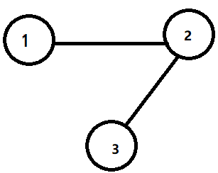
　　Here ,we can get something from the graph:

　　　　$A=\left[\begin{array}{ccc}0 & 1 & 0 \\1 & 0 & 1 \\0 & 1 & 0\end{array}\right]\quad D=\left[\begin{array}{ccc}1 & 0 & 0 \\0 & 2 & 0 \\0 & 0& 1\end{array}\right]\quad L=D-A=\left[\begin{array}{ccc}1 & -1 & 0 \\-1 & 2 & -1 \\0 & -1 & 1\end{array}\right]$

$K=0$ 时，卷积核为

　　　　$\begin{array}{l} g_{\theta}(\Lambda)&=\beta_{0} * T_{0}(\hat{L})\\&=\beta_{0} * I\\&=\left[\begin{array}{ccc}\beta_{0} & 0 & 0 \\0 & \beta_{0} & 0 \\0 & 0 & \beta_{0}\end{array}\right]\end{array}$

　　　　从这，发现 $K=0$ 时，可以发现此时卷积核只考虑了节点自身属性。

$K=1$ 时，卷积核为

　　　　$\begin{array}{l} g_{\theta}(\Lambda)&=\beta_{0} * T_{0}(\hat{L})+\beta_{1} * T_{1}(\hat{L})\\&=\left[\begin{array}{ccc}\beta_{0}+\beta_{1} & -\beta_{1} & 0 \\-\beta_{1} & \beta_{0}+2 \beta_{1} & -\beta_{1} \\0 & -\beta_{1} & \beta_{0}+\beta_{1}\end{array}\right]\end{array}$

　　　　从这，发现 $K=1$ 时，卷积核能关注到每个节点本身与其一阶相邻的节点。

$K=2$ 时，切比雪夫多项式 $T_{2}$ 为

　　　　$T_{2}(\hat{L})=2 \hat{L} T_{1}(\hat{L})-T_{0}(\hat{L}) $

　　此时卷积核为：

　　　　$\begin{array}{l} g_{\theta}(\Lambda)&=\beta_{0} * T_{0}(\hat{L})+\beta_{1} * T_{1}(\hat{L})+\beta_{2} * T_{2}(\hat{L}) \\&=\left[\begin{array}{ccc}\beta_{0}+\beta_{1}+3 \beta_{2} & -\beta_{1}-6 \beta_{2} & 2 \beta_{2} \\-\beta_{1}-6 \beta_{2} & \beta_{0}+2 \beta_{1}+11 \beta_{2} & -\beta_{1}-6 \beta_{2} \\2 \beta_{2} & -\beta_{1}-6 \beta_{2} & \beta_{0}+\beta_{1}+3 \beta_{2}\end{array}\right]\end{array}$

　　　　从这，发现 $K=2$ 时，卷积核能关注到每个节点本身与其一阶相邻和二阶相邻的节点。

$K=N$ 时，切比雪夫多项式 $T_{N}$ 为

　　　　$T_{N}(\hat{L})=2 \hat{L} T_{N-1}(\hat{L})-T_{N-2}(\hat{L})$

　　此时卷积核为

　　　　$g_{\theta}(\Lambda)=\sum\limits _{k=0}^{N} \beta_{k} T_{k}(\hat{\Lambda})$

　　　经过上面推导，可得 $K=N$ 能关注到每个节点本身与 $N$ 阶之内相邻的节点。

　　总结：

- 该卷积过程的复杂度为 $O(K|\varepsilon|)$ 。对比上一小节的多项式卷积核，这里利用切比雪夫多项式设计的卷积核只是利用仅包含加减操作的递归关系来计算 $T_{k}(\widetilde{L})$ ，这样大大减少了计算的复杂度。
- 参数共享机制：同阶共享相同参数，不同阶的参数不一样。

2.2 Layer-wise linear model

2.2.1 Application

　　Overfitting on local neighborhood structures：

- Graphs with very wide node degree distributions.

　　回忆 2.1.3 节中的切比雪夫多项式卷积核：

　　　　$g_{\theta}(\Lambda)=\sum\limits _{k=0}^{K} \beta_{k} T_{k}(\hat{\Lambda})$

　　此时图卷积为：（参考2.1.3节备注处）

　　　　$g*x=U g_{\theta}(\Lambda) U^{T} x=\sum\limits_{k=0}^{K} \beta_{k} T_{k}(\hat{L})x$

　　Where

- $\hat{L}=2 L / \lambda_{\max }-I$

　　为缓解上述 Overfitting on local neighborhood structures 问题，这里考虑 $K=1$ 和 $\lambda_{\max } \approx 2$ 的情况，即考虑自身属性与 $1$ 阶邻居属性。

　　则此时，图卷积 $g*x$ 简化为：

　　　　$\begin{array}{l} g*x&=\beta_{0} x+\beta_{1} \hat{L}x\\&=\beta_{0} x+\beta_{1}(2 L / \lambda_{\max }-I_{N})x\\&\approx \beta_{0} x+\beta_{1} (L-I_{N})x\\&\approx \beta_{0} x+\beta_{1} (L^{sym}-I_{N})x\\&=\beta_{0} x-\beta_{1} (D^{-\frac{1}{2}} A D^{-\frac{1}{2}})x\end{array}$

2.2.2 Simplification

　　我们设置 $\beta=\beta _{0}=-\beta_{1}$ ，得图卷积为
　　　　$g*x=\beta( I_{N}+D^{-\frac{1}{2}} A D^{-\frac{1}{2}} )x$

　　此时 $I_{N}+D^{-\frac{1}{2}} A D^{-\frac{1}{2}} $ 特征值的取值范围为 $[0,2]$。

　　 This operator can therefore lead to numerical instabilities and exploding/vanishing gradients when used in a deep neural network model.(带来梯度爆炸核梯度消失的问题)

　　所以采用下面的归一化技巧：

　　　　$I_{N}+D^{-\frac{1}{2}} A D^{-\frac{1}{2}} \rightarrow \tilde{D}^{-\frac{1}{2}} \tilde{A} \tilde{D}^{-\frac{1}{2}}$

　　Where

- $\tilde{A}=A+I_{N}$
- $\tilde{D}_{i i}=\sum_{j} \tilde{A}_{i j}$

2.2.3 Generalize above definition

　　考虑多通道输入的情况：

　　We can generalize this definition to a signal $X \in \mathbb{R}^{N \times C}$ with $C$ input channels (i.e. a $C$ -dimensional feature vector for every node) and $F$ filters or feature maps as follows:

　　　　$Z=\tilde{D}^{-\frac{1}{2}} \tilde{A} \tilde{D}^{-\frac{1}{2}} X \Theta$

　　where

- $\Theta \in \mathbb{R}^{C \times F}$ is now a matrix of filter parameters.(滤波器参数矩阵)
- $Z \in \mathbb{R}^{N \times F}$ is the convolved signal matrix.(卷积后的信号矩阵)

　　This filtering operation has complexity $\mathcal{O}(|\mathcal{E}| F C)$ , as $\tilde{A} X$ can be efficiently implemented as a product of a sparse matrix with a dense matrix.

3 Semi-supervised node classification

　　Flexible model $f(X, A)$ for efficient information propagation on graphs, we can return to the problem of semi-supervised node classification.

　　The overall model, a multi-layer GCN for semi-supervised learning, is schematically depicted in Figure 1.

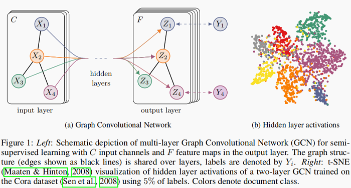
　　上图中，Figure 1 (a) 是一个 GCN 网络示意图，在 Input layer 拥有 $C$ 个输入，中间有若干隐藏层，在输出层有 $F$ 个特征映射；图的结构（边用黑线表示）在层之间共享；标签用$Y_{i}$表示。Figure 1(b)是一个两层 GCN 在 Cora 数据集上（使用了 5% 的标签）训练得到的隐藏层激活值的形象化表示，颜色表示文档类别。

3.1 Example

　　We consider a two-layer GCN for semi-supervised node classification on a graph with a symmetric adjacency matrix $A$ (binary or weighted).

　　Our forward model then takes the simple form

　　　　$Z=f(X, A)=\operatorname{softmax}\left(\hat{A} \operatorname{ReLU}\left(\hat{A} X W^{(0)}\right) W^{(1)}\right)$

　　Where

- $\hat{A}=\tilde{D}^{-\frac{1}{2}} \tilde{A} \tilde{D}^{-\frac{1}{2}}$ in a pre-processing step.
- $W^{(0)} \in \mathbb{R}^{C \times H}$ is an input-to-hidden weight matrix for a hidden layer with $H$ feature maps.
- $W^{(1)} \in \mathbb{R}^{H \times F}$ is a hidden-to-output weight matrix.
- Softmax activation function: $\operatorname{softmax}\left(x_{i}\right)=\frac{1}{\sum_{i} \exp \left(x_{i}\right)} \exp \left(x_{i}\right)$ with $\mathcal{Z}=\sum\limits _{i} \exp \left(x_{i}\right)$ , is applied row-wise.

　　For semi-supervised multiclass classification, we then evaluate the cross-entropy error over all labeled examples:

　　　　$\mathcal{L}=-\sum\limits _{l \in \mathcal{Y}_{L}} \sum\limits_{f=1}^{F} Y_{l f} \ln Z_{l f}$

　　Where

- $\mathcal{Y}_{L}$ is the set of node indices that have labels.
- The neural network weights $W_{(0)}$ and $W_{(1)}$ are trained using gradient descent.
- We perform batch gradient descent using the full dataset for every training iteration.
- Using a sparse representation for $A$, memory requirement is $O(|E|)$, i.e. linear in the number of edges.

4 Related work

　　略......

5 Experiments

　　Do some experiments:

semi-supervised document classification in citation networks;
semi-supervised entity classification in a bipartite graph extracted from a knowledge graph;
an evaluation of various graph propagation models;
a run-time analysis on random graphs.

5.1 Dayasets

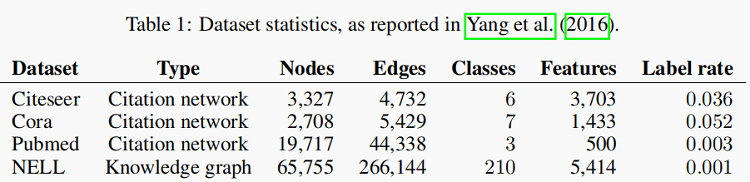
　　In the citation network datasets—Citeseer, Cora and Pubmed

- Nodes are documents.
- Edges are citation links.
- Label rate denotes the number of labeled nodes that are used for training divided by the total number of nodes in each dataset.

　　NELL is a bipartite graph dataset extracted from a knowledge graph with 55,864 relation nodes and 9,891 entity nodes.

5.2 Experimental set-up

We train a two-layer GCN as described in Section 3.1.
Evaluate prediction accuracy on a test set of 1,000 labeled examples.
We provide additional experiments using deeper models with up to 10 layers.
We choose the same dataset as in Yang et al. (2016) with an additional validation set of 500 labeled examples for hyperparameter optimization.

Dropout rate for all layers.
L2 regularization factor for the first GCN layer.
Number of hidden units.

5.3 Baselines

Label propagation (LP) (Zhu et al., 2003).
Semi-supervised embedding (SemiEmb) (Weston et al., 2012).
Manifold regularization (ManiReg) (Belkin et al., 2006) .
Skip-gram based graph embeddings (DeepWalk) (Perozzi et al., 2014).
Iterative classification algorithm (ICA) proposed in Lu & Getoor (2003).
Planetoid.

6 Results

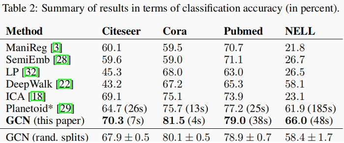
6.1 Semi-supervised node classification

　　 Results are summarized in Table 2.

6.2 Evaluation of propagation model

　　 We compare different variants of our proposed per-layer propagation model on the citation network datasets.

　　Results are summarized in Table 3.

　　The propagation model of our original GCN model is denoted by renormalization trick (in bold).

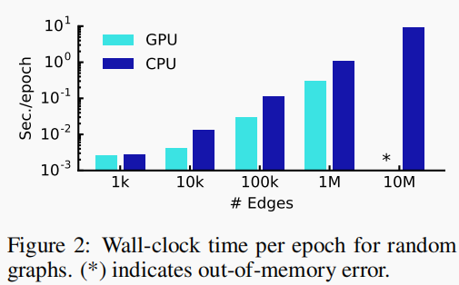
6.3 Training time per epoch

　　Here, we report results for the mean training time per epoch (forward pass, cross-entropy calculation, backward pass) for 100 epochs on simulated random graphs.

　　We compare results on a GPU and on a CPU-only.

　　Results are summarized in Figure 2.

7 Discussion

7.1 Semi-supervised model

　　Our model's advantage:

- Consider both nodes propertity and global structure.
- Easy to optimize.

7.2 Limitations and future work

Memory requirement.
Directed edges and edge features.
Limiting assumptions.

8 Conclusion

We have introduced a novel approach for semi-supervised classification on graph-structured data.
Our GCN model uses an efficient layer-wise propagation rule that is based on a first-order approximation of spectral convolutions on graphs.
The proposed GCN model is capable of encoding both graph structure and node features in a way useful for semi-supervised classification.
In this setting, our model outperforms several recently proposed methods by a significant margin, while being computationally efficient.