数据和特征决定了机器学习的上限,而模型和算法只是逼近这个上限而已
本文主要内容包括如下几点:
一、特征选择算法
具体介绍了:传统的特征选择算法(Wrapper methods、Filter methods、Embedded methods),以及:Laplacian Score拉普拉斯分数、Fisher Score等
二、数据降维算法
数据预处理(🐕特征选择和🐉数据降维度)原理以及python实现
一、特征选择(feature selection)
为什么要进行特征选择?
graph LR
B[input]-->A[ML]-->C[output]
观察上述流程图,假设\(input\)的数据特征为:{\(t_1...t_n\)}我们直接将输入投入到\(ML\)里面而后得到输出。但是问题来了,我们的特征\(t_1...t_n\)对于我们的\(output\)都有作用吗?
例子:定义我们的我们的\(ML\)为:男孩女孩判断模型,\(input\)的特征有:长/短头发、有/无喉结、邻居孩子男/女等,\(output\)为:男孩 or 女孩。
我相信很容易判断特征:邻居孩子男/女在对于我们模型效果上是不起作用的,那么的话在开始\(input\)时不添加该特征。
回归正题。特征选择(feature selection)作为一种数据预处理策略,在各种数据挖掘和机器学习问题准备数据(尤其是高维数据)方面是有效且高效的,特征选择的目标包括构建更简单、更易于理解的模型、提高数据挖掘性能以及准备干净、可理解的数据。
那么常用特征选择算法是什么呢?
1.1 传统特征选择算法
1.1.1 Wrapper method(包装法)
Wrapper methods rely on the predictive performance of a predefined learning algorithm to evaluate the quality of selected features.
wrapper方法依赖预先定义的学习算法的预测性能来评估所挑选特征的质量
算法步骤:
graph LR
A(挑选特征子集)-->B(评估挑选的特征)-->A
挑选特征子集,评估挑选特征直到合适为止
那么在Wrapper methods中对于特征子集的挑选就显得格外重要了,但是如若特征搜索空间为\(d\)那么就行搜索次数为\(2^d\),也就是说使用Wrapper methods很容易陷入NP-hard problem。两类参见的特征筛选方法:
定义全部特征为:\(Y=\{y_1...y_d\}\),定义输出特征:\(X_k=\{x_j|j=1,2...k;x_j\in Y\}\)
1、Sequential selection algorithms(SFS)
\[x^{+}=arg\ max\ J(X_k+x),\ x\in Y- X_k\\
X_k+1=X_k+x^+\\
k=k+1
\]
在空的特征子集中添加特征\(x\)使得目标函数\(J\)最大
- 2、Sequential Backward Selection(SBS)
\[x^-=arg\ max\ J(X_k-x),\ x\in X_k\\
X_{k-1}=X_k-x^-\\
k=k-1\\
\]
与SFS相类似,只不过SBS是从完整的特征开始,而后逐渐减少特征。
- 3、Sequential Floating Forward Selection (SFFS)
2、Heuristic Search Algorithms
算法步骤:首先初始化:\(X_0=\phi\),\(k=0\)
step1:
\[x^{+}=arg\ max\ J(X_k+x),\ x\in Y- X_k\\
X_k+1=X_k+x^+\\
k=k+1\\
go \ to \ step2
\]
在空的特征子集中添加特征\(x\)使得目标函数\(J\)最大
step2:
\[x^-=arg\ max\ J(X_k-x),\ x\in X_k\\
if\ J(X_k-x)>J(X_k)\\
X_{k-1}=X_k-x^-\\
k=k-1\\
go\ to\ step1
\]
SFFS较SFS多一个回溯操作(step2)
循环step1和step2只到达到目标\(k\)值停止。
!pip install mlxtend
from mlxtend.feature_selection import SequentialFeatureSelector as SFS
sfs = SFS(knn, #选择模型
          k_features=3, #选择筛选出的特征
          forward=True,
          floating=False,
          scoring='accuracy', #评价标准
          cv=4, #交叉验证
          n_jobs=-1 #用于并行评估不同特征子集的CPU数量,-1代表全部)
sfs = sfs.fit(X, y)
print(sbfs.k_feature_idx_) #返回选择的特征的序号 k_feature_names_返回特征名称
print(sbfs.k_score_) #返回评分
"""
forward与floating参数选择:
1、SFS算法True False
2、SBS算法False False
3、SFFS算法 True True
"""
2、Heuristic search algorithms 启发式搜索算法
Genetic Algorithm(GA)遗传算法
Wrapper methods缺点
1、计算代价高
2、容易过拟合
1.1.2 Filter methods(过滤法)
Filter methods use variable ranking techniques as the principle criteria for variable selection by ordering
Filter methods使用变量排序方法作为按顺序选择变量的原则标准
也就是说Fileter methods首先通过排序得到特征的相关性,而后进行筛选 !
算法步骤:
graph LR
A[特征重要性进行排序]-->B[将低特征滤出]
排序方法(ranking methods)
特征重要性计算有:
1、方差分析(ANOVA):基于统计方法来计算特征与目标变量之间的相关程度,通过计算特征的F值来评估特征的重要性。
2、互信息(Mutual Information):计算特征与目标变量之间的信息增益或互信息,衡量特征与目标变量之间的依赖关系。
如:通过信息增益进行评价
首先计算香农熵:
\[H(Y)=-\sum p(y)log(p(y))
\]
条件熵计算:
\[H(Y|X)=-\sum_{x} \sum_{y}p(x,y)log(p(y|x))
\]
而后计算:
\[I(Y,X)=H(Y)-H(Y|X)
\]
通过计算(3)就可以得到:如果\(X\)与\(Y\)之间相互独立那么将会趋近0
3、相关系数(Correlation Coefficient):计算特征和目标变量之间的线性相关性,常用的方法有Pearson相关系数和Spearman相关系数。
\[R(i)=\frac{cov(x_i,Y)}{\sqrt{var(x_i)*var(Y)}}
\]
其中\(Y\)作为输出变量(output)而\(x_i\)则为我们的input
4、卡方检验(Chi-square Test):针对分类问题,对特征和目标变量之间的关联程度进行检验,判断特征的重要性。
5、方差选择(Variance Threshold):通过计算特征的方差来判断其重要性,方差较低的特征可能对目标变量的预测作用较小
from sklearn.feature_selection import VarianceThreshold
X = [[0, 0, 1], [0, 1, 0], [1, 0, 0], [0, 1, 1], [0, 1, 0], [0, 1, 1]]
sel = VarianceThreshold(threshold=(.8 * (1 - .8))) #threshold指定特征选择的方法
sel.fit_transform(X)
"""
array([[0, 1],
       [1, 0],
       [0, 0],
       [1, 1],
       [1, 0],
       [1, 1]])
""""
参数说明:
sklearn-filter methods
1.1.3 Embedded methods(嵌入法)
Embedded methods is a tradeoff between filter and wrapper methods that embed the feature selection into model learning.
Embedded方法将Wrapped和filter方法进行权衡,将特征选择嵌入到模型学习中去
1.2 其它特征选择方法
基于信息论:一般是指通过计算信息增益等来表示特征重要性
基于相似:主要通过计算特征体系中的各特征之间的“相似”。比如无监督特征选择:可以通过计算各自特征样本之间距离(距离近则相似);而对于监督特征选择一般则是通过标签信息得到(比如可以计算相关矩阵等)
1.2.1 Laplacian Score 拉普拉斯分数
HE X, CAI D, NIYOGI P. Laplacian Score for Feature Selection[C/OL]//Advances in Neural Information Processing Systems: 卷 18. MIT Press, 2005[2023-07-07].
原文描述如下:
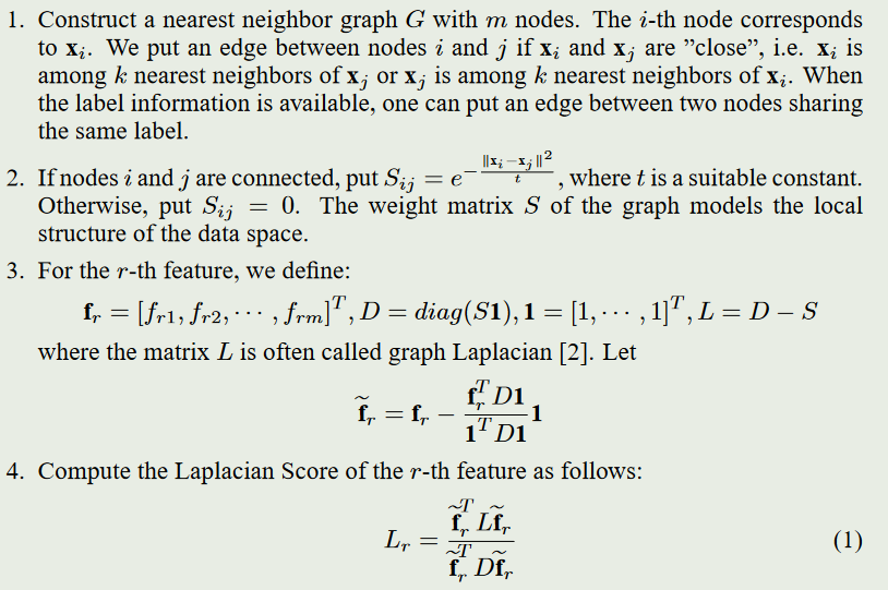
解释如下:
\(f_{ri}\)代表第\(r\)个特征的第\(i\)个样本;
-
构建图(Graph):首先,需要构建一个图\(G\),其中节点(\(m\)个节点)代表样本数据的特征,边代表特征之间的相似度或关联关系。常用的方法是使用K近邻来构建图,即对每个特征找到K个最近的邻居,并将它们连接起来。
-
计算亲和矩阵(Affinity Matrix):在构建了图之后,需要计算特征之间的相似度或关联性。节点之间彼此连接时通过使用:\(S(i,j)=e^{-\frac{||x_i-x_j||^2}{t}}\),其中\(x_i\)为\(x_j\)的\(p\)个最相邻的节点,\(t\)为常数。如果节点之间不相互连接那么\(S(i,j)=0\)
\(S_{ij}\)较大,说明节点比较“接近”
-
计算拉普拉斯矩阵(Laplacian Matrix):首先定义对角矩阵D(diagonal matrix D):\(D(i,j)=\sum_{j=1}^{n}S(i,j)\)。那么拉普拉斯矩阵为:\(L=D-S\)。
-
计算每个特征的拉普拉斯分数(Laplacian Score):
\[L_r=\frac{\widetilde{f}_{r}^{T}L\widetilde{f_r}}{\widetilde{f}_{r}^{T}D\widetilde{f}_r}
\]
其中:\(\widetilde{f_r}=f_r-\frac{f_r^TD1}{1^TD1}1\)、\(1=[1,...,1]^T\)、\(f_r=[f_{r1},...,f_{rm}]^T\)、\(D=diag(S1)\)
- 选择k个特征的任务可以通过选择具有最小拉普拉斯分数的前k个特征来解决
代码如下:
详细代码
```python
import numpy as np
from scipy.sparse import *
from sklearn.metrics.pairwise import pairwise_distances
def lap_score(X, **kwargs):
"""
This function implements the laplacian score feature selection, steps are as follows:
1. Construct the affinity matrix W if it is not specified
2. For the r-th feature, we define fr = X(:,r), D = diag(W*ones), ones = [1,...,1]', L = D - W
3. Let fr_hat = fr - (fr'*D*ones)*ones/(ones'*D*ones)
4. Laplacian score for the r-th feature is score = (fr_hat'*L*fr_hat)/(fr_hat'*D*fr_hat)
Input
-----
X: {numpy array}, shape (n_samples, n_features)
input data
kwargs: {dictionary}
W: {sparse matrix}, shape (n_samples, n_samples)
input affinity matrix
Output
------
score: {numpy array}, shape (n_features,)
laplacian score for each feature
Reference
---------
He, Xiaofei et al. "Laplacian Score for Feature Selection." NIPS 2005.
"""
# if 'W' is not specified, use the default W
if 'W' not in kwargs.keys():
W = construct_W(X)
# construct the affinity matrix W
W = kwargs['W']
# build the diagonal D matrix from affinity matrix W
D = np.array(W.sum(axis=1))
L = W
tmp = np.dot(np.transpose(D), X)
D = diags(np.transpose(D), [0])
Xt = np.transpose(X)
t1 = np.transpose(np.dot(Xt, D.todense()))
t2 = np.transpose(np.dot(Xt, L.todense()))
# compute the numerator of Lr
D_prime = np.sum(np.multiply(t1, X), 0) - np.multiply(tmp, tmp)/D.sum()
# compute the denominator of Lr
L_prime = np.sum(np.multiply(t2, X), 0) - np.multiply(tmp, tmp)/D.sum()
# avoid the denominator of Lr to be 0
D_prime[D_prime < 1e-12] = 10000
# compute laplacian score for all features
score = 1 - np.array(np.multiply(L_prime, 1/D_prime))[0, :]
return np.transpose(score)
def feature_ranking(score):
"""
Rank features in ascending order according to their laplacian scores, the smaller the laplacian score is, the more
important the feature is
"""
idx = np.argsort(score, 0)
return idx
def construct_W(X, **kwargs):
"""
Construct the affinity matrix W through different ways
Notes
-----
if kwargs is null, use the default parameter settings;
if kwargs is not null, construct the affinity matrix according to parameters in kwargs
Input
-----
X: {numpy array}, shape (n_samples, n_features)
input data
kwargs: {dictionary}
parameters to construct different affinity matrix W:
y: {numpy array}, shape (n_samples, 1)
the true label information needed under the 'supervised' neighbor mode
metric: {string}
choices for different distance measures
'euclidean' - use euclidean distance
'cosine' - use cosine distance (default)
neighbor_mode: {string}
indicates how to construct the graph
'knn' - put an edge between two nodes if and only if they are among the
k nearest neighbors of each other (default)
'supervised' - put an edge between two nodes if they belong to same class
and they are among the k nearest neighbors of each other
weight_mode: {string}
indicates how to assign weights for each edge in the graph
'binary' - 0-1 weighting, every edge receives weight of 1 (default)
'heat_kernel' - if nodes i and j are connected, put weight W_ij = exp(-norm(x_i - x_j)/2t^2)
this weight mode can only be used under 'euclidean' metric and you are required
to provide the parameter t
'cosine' - if nodes i and j are connected, put weight cosine(x_i,x_j).
this weight mode can only be used under 'cosine' metric
k: {int}
choices for the number of neighbors (default k = 5)
t: {float}
parameter for the 'heat_kernel' weight_mode
fisher_score: {boolean}
indicates whether to build the affinity matrix in a fisher score way, in which W_ij = 1/n_l if yi = yj = l;
otherwise W_ij = 0 (default fisher_score = false)
reliefF: {boolean}
indicates whether to build the affinity matrix in a reliefF way, NH(x) and NM(x,y) denotes a set of
k nearest points to x with the same class as x, and a different class (the class y), respectively.
W_ij = 1 if i = j; W_ij = 1/k if x_j \in NH(x_i); W_ij = -1/(c-1)k if x_j \in NM(x_i, y) (default reliefF = false)
Output
------
W: {sparse matrix}, shape (n_samples, n_samples)
output affinity matrix W
"""
# default metric is 'cosine'
if 'metric' not in kwargs.keys():
kwargs['metric'] = 'cosine'
# default neighbor mode is 'knn' and default neighbor size is 5
if 'neighbor_mode' not in kwargs.keys():
kwargs['neighbor_mode'] = 'knn'
if kwargs['neighbor_mode'] == 'knn' and 'k' not in kwargs.keys():
kwargs['k'] = 5
if kwargs['neighbor_mode'] == 'supervised' and 'k' not in kwargs.keys():
kwargs['k'] = 5
if kwargs['neighbor_mode'] == 'supervised' and 'y' not in kwargs.keys():
print ('Warning: label is required in the supervised neighborMode!!!')
exit(0)
# default weight mode is 'binary', default t in heat kernel mode is 1
if 'weight_mode' not in kwargs.keys():
kwargs['weight_mode'] = 'binary'
if kwargs['weight_mode'] == 'heat_kernel':
if kwargs['metric'] != 'euclidean':
kwargs['metric'] = 'euclidean'
if 't' not in kwargs.keys():
kwargs['t'] = 1
elif kwargs['weight_mode'] == 'cosine':
if kwargs['metric'] != 'cosine':
kwargs['metric'] = 'cosine'
# default fisher_score and reliefF mode are 'false'
if 'fisher_score' not in kwargs.keys():
kwargs['fisher_score'] = False
if 'reliefF' not in kwargs.keys():
kwargs['reliefF'] = False
n_samples, n_features = np.shape(X)
# choose 'knn' neighbor mode
if kwargs['neighbor_mode'] == 'knn':
k = kwargs['k']
if kwargs['weight_mode'] == 'binary':
if kwargs['metric'] == 'euclidean':
# compute pairwise euclidean distances
D = pairwise_distances(X)
D **= 2
# sort the distance matrix D in ascending order
dump = np.sort(D, axis=1)
idx = np.argsort(D, axis=1)
# choose the k-nearest neighbors for each instance
idx_new = idx[:, 0:k+1]
G = np.zeros((n_samples*(k+1), 3))
G[:, 0] = np.tile(np.arange(n_samples), (k+1, 1)).reshape(-1)
G[:, 1] = np.ravel(idx_new, order='F')
G[:, 2] = 1
# build the sparse affinity matrix W
W = csc_matrix((G[:, 2], (G[:, 0], G[:, 1])), shape=(n_samples, n_samples))
bigger = np.transpose(W) > W
W = W - W.multiply(bigger) + np.transpose(W).multiply(bigger)
return W
elif kwargs['metric'] == 'cosine':
# normalize the data first
X_normalized = np.power(np.sum(X*X, axis=1), 0.5)
for i in range(n_samples):
X[i, :] = X[i, :]/max(1e-12, X_normalized[i])
# compute pairwise cosine distances
D_cosine = np.dot(X, np.transpose(X))
# sort the distance matrix D in descending order
dump = np.sort(-D_cosine, axis=1)
idx = np.argsort(-D_cosine, axis=1)
idx_new = idx[:, 0:k+1]
G = np.zeros((n_samples*(k+1), 3))
G[:, 0] = np.tile(np.arange(n_samples), (k+1, 1)).reshape(-1)
G[:, 1] = np.ravel(idx_new, order='F')
G[:, 2] = 1
# build the sparse affinity matrix W
W = csc_matrix((G[:, 2], (G[:, 0], G[:, 1])), shape=(n_samples, n_samples))
bigger = np.transpose(W) > W
W = W - W.multiply(bigger) + np.transpose(W).multiply(bigger)
return W
elif kwargs['weight_mode'] == 'heat_kernel':
t = kwargs['t']
# compute pairwise euclidean distances
D = pairwise_distances(X)
D **= 2
# sort the distance matrix D in ascending order
dump = np.sort(D, axis=1)
idx = np.argsort(D, axis=1)
idx_new = idx[:, 0:k+1]
dump_new = dump[:, 0:k+1]
# compute the pairwise heat kernel distances
dump_heat_kernel = np.exp(-dump_new/(2*t*t))
G = np.zeros((n_samples*(k+1), 3))
G[:, 0] = np.tile(np.arange(n_samples), (k+1, 1)).reshape(-1)
G[:, 1] = np.ravel(idx_new, order='F')
G[:, 2] = np.ravel(dump_heat_kernel, order='F')
# build the sparse affinity matrix W
W = csc_matrix((G[:, 2], (G[:, 0], G[:, 1])), shape=(n_samples, n_samples))
bigger = np.transpose(W) > W
W = W - W.multiply(bigger) + np.transpose(W).multiply(bigger)
return W
elif kwargs['weight_mode'] == 'cosine':
# normalize the data first
X_normalized = np.power(np.sum(X*X, axis=1), 0.5)
for i in range(n_samples):
X[i, :] = X[i, :]/max(1e-12, X_normalized[i])
# compute pairwise cosine distances
D_cosine = np.dot(X, np.transpose(X))
# sort the distance matrix D in ascending order
dump = np.sort(-D_cosine, axis=1)
idx = np.argsort(-D_cosine, axis=1)
idx_new = idx[:, 0:k+1]
dump_new = -dump[:, 0:k+1]
G = np.zeros((n_samples*(k+1), 3))
G[:, 0] = np.tile(np.arange(n_samples), (k+1, 1)).reshape(-1)
G[:, 1] = np.ravel(idx_new, order='F')
G[:, 2] = np.ravel(dump_new, order='F')
# build the sparse affinity matrix W
W = csc_matrix((G[:, 2], (G[:, 0], G[:, 1])), shape=(n_samples, n_samples))
bigger = np.transpose(W) > W
W = W - W.multiply(bigger) + np.transpose(W).multiply(bigger)
return W
# choose supervised neighborMode
elif kwargs['neighbor_mode'] == 'supervised':
k = kwargs['k']
# get true labels and the number of classes
y = kwargs['y']
label = np.unique(y)
n_classes = np.unique(y).size
# construct the weight matrix W in a fisherScore way, W_ij = 1/n_l if yi = yj = l, otherwise W_ij = 0
if kwargs['fisher_score'] is True:
W = lil_matrix((n_samples, n_samples))
for i in range(n_classes):
class_idx = (y == label[i])
class_idx_all = (class_idx[:, np.newaxis] & class_idx[np.newaxis, :])
W[class_idx_all] = 1.0/np.sum(np.sum(class_idx))
return W
# construct the weight matrix W in a reliefF way, NH(x) and NM(x,y) denotes a set of k nearest
# points to x with the same class as x, a different class (the class y), respectively. W_ij = 1 if i = j;
# W_ij = 1/k if x_j \in NH(x_i); W_ij = -1/(c-1)k if x_j \in NM(x_i, y)
if kwargs['reliefF'] is True:
# when xj in NH(xi)
G = np.zeros((n_samples*(k+1), 3))
id_now = 0
for i in range(n_classes):
class_idx = np.column_stack(np.where(y == label[i]))[:, 0]
D = pairwise_distances(X[class_idx, :])
D **= 2
idx = np.argsort(D, axis=1)
idx_new = idx[:, 0:k+1]
n_smp_class = (class_idx[idx_new[:]]).size
if len(class_idx) <= k:
k = len(class_idx) - 1
G[id_now:n_smp_class+id_now, 0] = np.tile(class_idx, (k+1, 1)).reshape(-1)
G[id_now:n_smp_class+id_now, 1] = np.ravel(class_idx[idx_new[:]], order='F')
G[id_now:n_smp_class+id_now, 2] = 1.0/k
id_now += n_smp_class
W1 = csc_matrix((G[:, 2], (G[:, 0], G[:, 1])), shape=(n_samples, n_samples))
# when i = j, W_ij = 1
for i in range(n_samples):
W1[i, i] = 1
# when x_j in NM(x_i, y)
G = np.zeros((n_samples*k*(n_classes - 1), 3))
id_now = 0
for i in range(n_classes):
class_idx1 = np.column_stack(np.where(y == label[i]))[:, 0]
X1 = X[class_idx1, :]
for j in range(n_classes):
if label[j] != label[i]:
class_idx2 = np.column_stack(np.where(y == label[j]))[:, 0]
X2 = X[class_idx2, :]
D = pairwise_distances(X1, X2)
idx = np.argsort(D, axis=1)
idx_new = idx[:, 0:k]
n_smp_class = len(class_idx1)*k
G[id_now:n_smp_class+id_now, 0] = np.tile(class_idx1, (k, 1)).reshape(-1)
G[id_now:n_smp_class+id_now, 1] = np.ravel(class_idx2[idx_new[:]], order='F')
G[id_now:n_smp_class+id_now, 2] = -1.0/((n_classes-1)*k)
id_now += n_smp_class
W2 = csc_matrix((G[:, 2], (G[:, 0], G[:, 1])), shape=(n_samples, n_samples))
bigger = np.transpose(W2) > W2
W2 = W2 - W2.multiply(bigger) + np.transpose(W2).multiply(bigger)
W = W1 + W2
return W
if kwargs['weight_mode'] == 'binary':
if kwargs['metric'] == 'euclidean':
G = np.zeros((n_samples*(k+1), 3))
id_now = 0
for i in range(n_classes):
class_idx = np.column_stack(np.where(y == label[i]))[:, 0]
# compute pairwise euclidean distances for instances in class i
D = pairwise_distances(X[class_idx, :])
D **= 2
# sort the distance matrix D in ascending order for instances in class i
idx = np.argsort(D, axis=1)
idx_new = idx[:, 0:k+1]
n_smp_class = len(class_idx)*(k+1)
G[id_now:n_smp_class+id_now, 0] = np.tile(class_idx, (k+1, 1)).reshape(-1)
G[id_now:n_smp_class+id_now, 1] = np.ravel(class_idx[idx_new[:]], order='F')
G[id_now:n_smp_class+id_now, 2] = 1
id_now += n_smp_class
# build the sparse affinity matrix W
W = csc_matrix((G[:, 2], (G[:, 0], G[:, 1])), shape=(n_samples, n_samples))
bigger = np.transpose(W) > W
W = W - W.multiply(bigger) + np.transpose(W).multiply(bigger)
return W
if kwargs['metric'] == 'cosine':
# normalize the data first
X_normalized = np.power(np.sum(X*X, axis=1), 0.5)
for i in range(n_samples):
X[i, :] = X[i, :]/max(1e-12, X_normalized[i])
G = np.zeros((n_samples*(k+1), 3))
id_now = 0
for i in range(n_classes):
class_idx = np.column_stack(np.where(y == label[i]))[:, 0]
# compute pairwise cosine distances for instances in class i
D_cosine = np.dot(X[class_idx, :], np.transpose(X[class_idx, :]))
# sort the distance matrix D in descending order for instances in class i
idx = np.argsort(-D_cosine, axis=1)
idx_new = idx[:, 0:k+1]
n_smp_class = len(class_idx)*(k+1)
G[id_now:n_smp_class+id_now, 0] = np.tile(class_idx, (k+1, 1)).reshape(-1)
G[id_now:n_smp_class+id_now, 1] = np.ravel(class_idx[idx_new[:]], order='F')
G[id_now:n_smp_class+id_now, 2] = 1
id_now += n_smp_class
# build the sparse affinity matrix W
W = csc_matrix((G[:, 2], (G[:, 0], G[:, 1])), shape=(n_samples, n_samples))
bigger = np.transpose(W) > W
W = W - W.multiply(bigger) + np.transpose(W).multiply(bigger)
return W
elif kwargs['weight_mode'] == 'heat_kernel':
G = np.zeros((n_samples*(k+1), 3))
id_now = 0
for i in range(n_classes):
class_idx = np.column_stack(np.where(y == label[i]))[:, 0]
# compute pairwise cosine distances for instances in class i
D = pairwise_distances(X[class_idx, :])
D **= 2
# sort the distance matrix D in ascending order for instances in class i
dump = np.sort(D, axis=1)
idx = np.argsort(D, axis=1)
idx_new = idx[:, 0:k+1]
dump_new = dump[:, 0:k+1]
t = kwargs['t']
# compute pairwise heat kernel distances for instances in class i
dump_heat_kernel = np.exp(-dump_new/(2*t*t))
n_smp_class = len(class_idx)*(k+1)
G[id_now:n_smp_class+id_now, 0] = np.tile(class_idx, (k+1, 1)).reshape(-1)
G[id_now:n_smp_class+id_now, 1] = np.ravel(class_idx[idx_new[:]], order='F')
G[id_now:n_smp_class+id_now, 2] = np.ravel(dump_heat_kernel, order='F')
id_now += n_smp_class
# build the sparse affinity matrix W
W = csc_matrix((G[:, 2], (G[:, 0], G[:, 1])), shape=(n_samples, n_samples))
bigger = np.transpose(W) > W
W = W - W.multiply(bigger) + np.transpose(W).multiply(bigger)
return W
elif kwargs['weight_mode'] == 'cosine':
# normalize the data first
X_normalized = np.power(np.sum(X*X, axis=1), 0.5)
for i in range(n_samples):
X[i, :] = X[i, :]/max(1e-12, X_normalized[i])
G = np.zeros((n_samples*(k+1), 3))
id_now = 0
for i in range(n_classes):
class_idx = np.column_stack(np.where(y == label[i]))[:, 0]
# compute pairwise cosine distances for instances in class i
D_cosine = np.dot(X[class_idx, :], np.transpose(X[class_idx, :]))
# sort the distance matrix D in descending order for instances in class i
dump = np.sort(-D_cosine, axis=1)
idx = np.argsort(-D_cosine, axis=1)
idx_new = idx[:, 0:k+1]
dump_new = -dump[:, 0:k+1]
n_smp_class = len(class_idx)*(k+1)
G[id_now:n_smp_class+id_now, 0] = np.tile(class_idx, (k+1, 1)).reshape(-1)
G[id_now:n_smp_class+id_now, 1] = np.ravel(class_idx[idx_new[:]], order='F')
G[id_now:n_smp_class+id_now, 2] = np.ravel(dump_new, order='F')
id_now += n_smp_class
# build the sparse affinity matrix W
W = csc_matrix((G[:, 2], (G[:, 0], G[:, 1])), shape=(n_samples, n_samples))
bigger = np.transpose(W) > W
W = W - W.multiply(bigger) + np.transpose(W).multiply(bigger)
return W
import pandas as pd
from sklearn.model_selection import train_test_split #数据集划分
data = pd.read_excel(r'path')
data = data.drop(data[data['PM10']=='—'].index) #去除缺失数据
data.head()
x = data.iloc[:,7:]
y = data['AQI']
X_train, X_test, y_train, y_test = train_test_split(x, y, test_size=0.2, random_state=40)
kwargs_W = {"metric":"euclidean","neighbor_mode":"knn","weight_mode":"heat_kernel","k":5,'t':1}
W = construct_W(x, **kwargs_W)
score = lap_score(x.values, W=W)
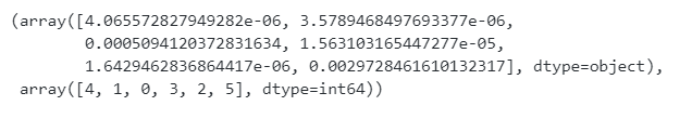
idx = feature_ranking(score)
score, idx
```
代码运行结果:
1.2.2 Fisher Score
Fisher Score是一种监督特征选取算法,通过挑选特征使得同一样本中特征值相似,不同类别特征值不相似。计算公式如下:
\[f_i=\frac{\sum_{j=1}^{c}n_j(\mu_{ij}-\mu_i)^2}{\sum_{j=1}^{c}n_j\sigma_{ij}^{2}}
\]
其中\(n_j\)代表类别\(j\)的数量、\(\mu_{ij}\)代表\(j\)类样本特征\(f_i\)的平均值、\(\mu_j\)代笔特征\(f_i\)的平均值
1.3 总结
二、数据降维
为什么要进行数据降维度?数据维度又是什么?
数据降维:将高维空间数据投影到低维空间,目的在于将数据的特征维度降低,作用和特征筛选的作用相类似但是两种之间有一定区别(两者都属于降低数据维度方法):
数据降维和特征筛选:两者都是对数据的维度进行减少,但是特征筛选:侧重在于从\(D\)维特征从选择\(d\)维特征,数据特征个数发生减少;数据降维:从高维向低维投影;通俗易懂描述为:前者为阉割(数量变化),后者为压缩("形状"变化)
数据降维分类:
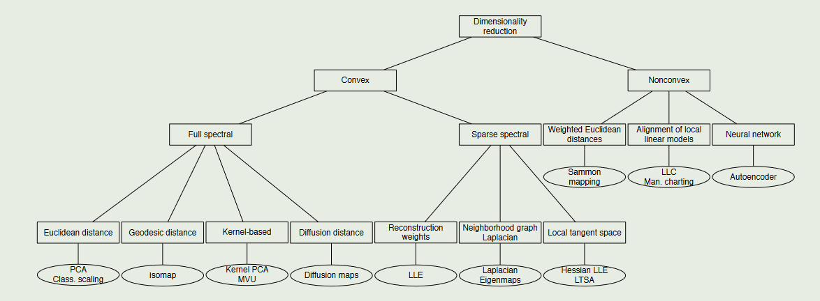
2.1 Principal Components Analysis(PCA)主成分分析
PCA是一种线性降维技术,即通过将数据嵌入到较低维的线性子空间中来进行降维。
PCA通过寻找低维数据对高维数据进行描述
数学原理如下:对于原始数据\(X\)通过找到映射\(M\)将原始数据从较高维度的\(D\)维转化为较低维度的\(d\)维即:\(Y=XM\)(\(Y\)代表转化后的低维数据),那么问题关键在于对于映射\(M\)的寻找.
PCA算法流程:
1、对输入数据\(X=\{x_1...x_n\}\)进行中心化:$x_i=x_i- \frac{1}{m}\sum_{j=1}^{n}x_j \(
2、对中心化的数据计算协方差矩阵:\)X^TX\(
3、计算协方差矩阵特征值,并且得到最大的\)n{'}$($n\(代表要降低到的维度)个特征值所对应特征向量:\)M=(w_1..w_{n^{'}})\(
4、对样本进行转换:\)Y=XM$
from sklearn.decomposition import PCA
x = np.random.randn(10,5)
pca = PCA(3)
pca.fit(x)
pca.transform(x) #转化
pca.explained_variance_ratio_ #贡献
参考文献
[1] LI J, CHENG K, WANG S, 等. Feature Selection:A Data Perspective[J/OL]. ACM Computing Surveys, 2018, 50(6): 1-45. https://doi.org/10.1145/3136625.
[2]CHANDRASHEKAR G, SAHIN F. A survey on feature selection methods[J/OL]. Computers & Electrical Engineering, 2014, 40(1): 16-28. DOI:10.1016/j.compeleceng.2013.11.024.
[3]https://rasbt.github.io/mlxtend/user_guide/feature_selection/SequentialFeatureSelector/
[4]Van Der Maaten, Laurens, Eric Postma, and Jaap Van den Herik."Dimensionality reduction:a comparative." J Mach Learn Res 10.66-71 (2009).
[5]HE X, CAI D, NIYOGI P.Laplacian Score for Feature Selection[C/OL]//Advances in Neural Information Processing Systems: 卷 18. MIT Press, 2005[2023-07-07].
推荐阅读
⭐⭐⭐LI J, CHENG K, WANG S, 等. Feature Selection: A Data Perspective[J/OL]. ACM Computing Surveys, 2018, 50(6): 1-45. https://doi.org/10.1145/3136625.
⭐⭐Van Der Maaten, Laurens, Eric Postma, and Jaap Van den Herik."Dimensionality reduction:a comparative." J Mach Learn Res 10.66-71 (2009).


 浙公网安备 33010602011771号