

TensorFlow读书笔记
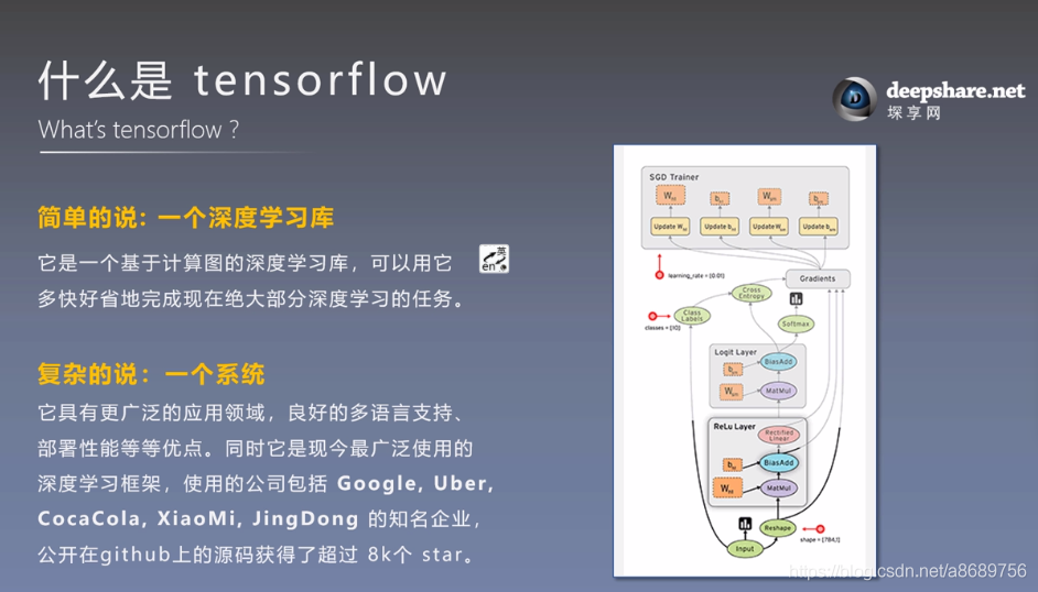
1.TensorFlow介绍
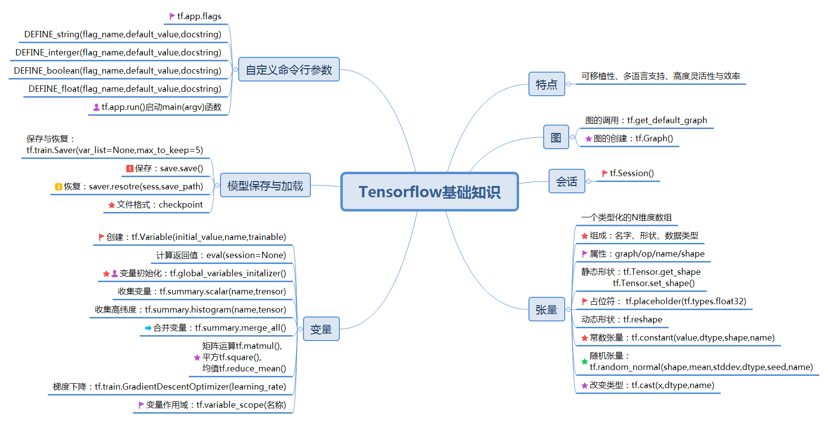
2.TensorFlow基础知识
备注:
- 使用
图 (graph)来表示计算任务. - 在被称之为
会话 (Session)的上下文 (context) 中执行图. - 使用 tensor 表示数据.
- 通过
变量 (Variable)维护状态. - 使用 feed 和 fetch 可以为任意的操作(arbitrary operation) 赋值或者从其中获取数据
3.TensorFlow的五个主要特征
高度的灵活性
TensorFlow 不是一个严格的“神经网络”库。只要你可以将你的计算表示为一个数据流图,你就可以使用Tensorflow。你来构建图,描写驱动计算的内部循环。我们提供了有用的工具来帮助你组装“子图”(常用于神经网络),当然用户也可以自己在Tensorflow基础上写自己的“上层库”。定义顺手好用的新复合操作和写一个python函数一样容易,而且也不用担心性能损耗。当然万一你发现找不到想要的底层数据操作,你也可以自己写一点c++代码来丰富底层的操作。
真正的可移植性(Portability)
Tensorflow 在CPU和GPU上运行,比如说可以运行在台式机、服务器、手机移动设备等等。想要在没有特殊硬件的前提下,在你的笔记本上跑一下机器学习的新想法?Tensorflow可以办到这点。准备将你的训练模型在多个CPU上规模化运算,又不想修改代码?Tensorflow可以办到这点。想要将你的训练好的模型作为产品的一部分用到手机app里?Tensorflow可以办到这点。你改变主意了,想要将你的模型作为云端服务运行在自己的服务器上,或者运行在Docker容器里?Tensorfow也能办到
多语言支持
Tensorflow 有一个合理的c++使用界面,也有一个易用的python使用界面来构建和执行你的graphs。你可以直接写python/c++程序,也可以用交互式的ipython界面来用Tensorflow尝试些想法,它可以帮你将笔记、代码、可视化等有条理地归置好。当然这仅仅是个起点——我们希望能鼓励你创造自己最喜欢的语言界面,比如Go,Java,Lua,Javascript,或者是R
性能最优化
比如说你又一个32个CPU内核、4个GPU显卡的工作站,想要将你工作站的计算潜能全发挥出来?由于Tensorflow 给予了线程、队列、异步操作等以最佳的支持,Tensorflow 让你可以将你手边硬件的计算潜能全部发挥出来。你可以自由地将Tensorflow图中的计算元素分配到不同设备上,Tensorflow可以帮你管理好这些不同副本。
4.TensorFlow基础入门
# 安装 TensorFlow

import tensorflow as tf
#载入并准备好 MNIST 数据集。将样本从整数转换为浮点数:
mnist = tf.keras.datasets.mnist

(x_train, y_train), (x_test, y_test) = mnist.load_data()
x_train, x_test = x_train / 255.0, x_test / 255.0

#将模型的各层堆叠起来,以搭建 tf.keras.Sequential 模型。为训练选择优化器和损失函数:
model = tf.keras.models.Sequential([
  tf.keras.layers.Flatten(input_shape=(28, 28)),
  tf.keras.layers.Dense(128, activation='relu'),
  tf.keras.layers.Dropout(0.2),
  tf.keras.layers.Dense(10, activation='softmax')
])

model.compile(optimizer='adam',
              loss='sparse_categorical_crossentropy',
              metrics=['accuracy'])
#训练并验证模型
model.fit(x_train, y_train, epochs=5)

model.evaluate(x_test,  y_test, verbose=2)
结果:
Epoch 1/5
1875/1875 [==============================] - 3s 2ms/step - loss: 0.2962 - accuracy: 0.9155
Epoch 2/5
1875/1875 [==============================] - 3s 2ms/step - loss: 0.1420 - accuracy: 0.9581
Epoch 3/5
1875/1875 [==============================] - 3s 2ms/step - loss: 0.1064 - accuracy: 0.9672
Epoch 4/5
1875/1875 [==============================] - 3s 2ms/step - loss: 0.0885 - accuracy: 0.9730
Epoch 5/5
1875/1875 [==============================] - 3s 2ms/step - loss: 0.0749 - accuracy: 0.9765
313/313 - 0s - loss: 0.0748 - accuracy: 0.9778
[0.07484959065914154, 0.9778000116348267]
5.TensorFlow练习
1.服装图像分类
# TensorFlow and tf.keras
import tensorflow as tf
from tensorflow import keras
# Helper libraries
import numpy as np
import matplotlib.pyplot as plt
print(tf.__version__)
fashion_mnist = keras.datasets.fashion_mnist
(train_images, train_labels), (test_images, test_labels) = fashion_mnist.load_data()
class_names = ['T-shirt/top', 'Trouser', 'Pullover', 'Dress', 'Coat',
'Sandal', 'Shirt', 'Sneaker', 'Bag', 'Ankle boot']
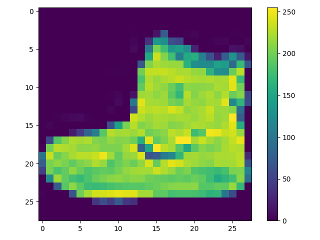
plt.figure()
plt.imshow(train_images[0])
plt.colorbar()
plt.grid(False)
plt.show()
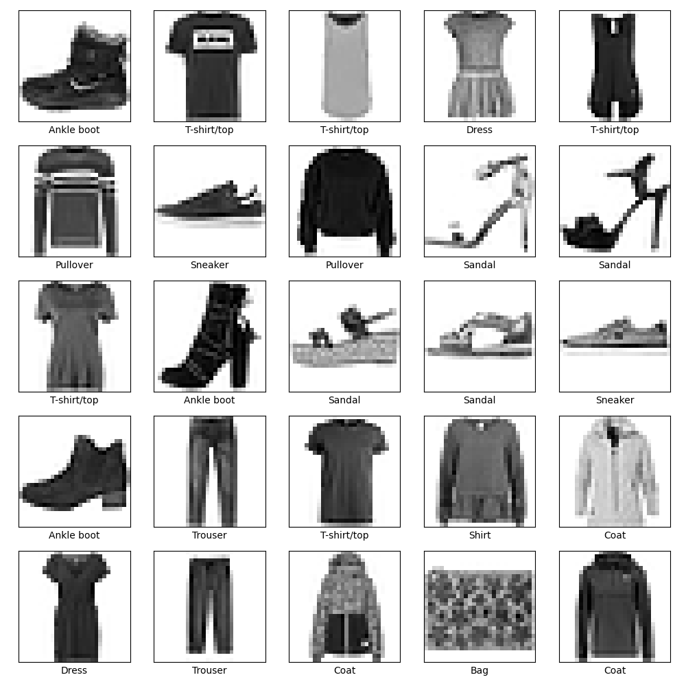
train_images = train_images / 255.0
test_images = test_images / 255.0
plt.figure(figsize=(10,10))
for i in range(25):
plt.subplot(5,5,i+1)
plt.xticks([])
plt.yticks([])
plt.grid(False)
plt.imshow(train_images[i], cmap=plt.cm.binary)
plt.xlabel(class_names[train_labels[i]])
plt.show()
model = keras.Sequential([
keras.layers.Flatten(input_shape=(28, 28)),
keras.layers.Dense(128, activation='relu'),
keras.layers.Dense(10)
])
model.compile(optimizer='adam',
loss=tf.keras.losses.SparseCategoricalCrossentropy(from_logits=True),
metrics=['accuracy'])
model.fit(train_images, train_labels, epochs=10)
test_loss, test_acc = model.evaluate(test_images, test_labels, verbose=2)
print('\nTest accuracy:', test_acc)
probability_model = tf.keras.Sequential([model,
tf.keras.layers.Softmax()])
predictions = probability_model.predict(test_images)
np.argmax(predictions[0])
def plot_image(i, predictions_array, true_label, img):
predictions_array, true_label, img = predictions_array, true_label[i], img[i]
plt.grid(False)
plt.xticks([])
plt.yticks([])
plt.imshow(img, cmap=plt.cm.binary)
predicted_label = np.argmax(predictions_array)
if predicted_label == true_label:
color = 'blue'
else:
color = 'red'
plt.xlabel("{} {:2.0f}% ({})".format(class_names[predicted_label],
100*np.max(predictions_array),
class_names[true_label]),
color=color)
def plot_value_array(i, predictions_array, true_label):
predictions_array, true_label = predictions_array, true_label[i]
plt.grid(False)
plt.xticks(range(10))
plt.yticks([])
thisplot = plt.bar(range(10), predictions_array, color="#777777")
plt.ylim([0, 1])
predicted_label = np.argmax(predictions_array)
thisplot[predicted_label].set_color('red')
thisplot[true_label].set_color('blue')
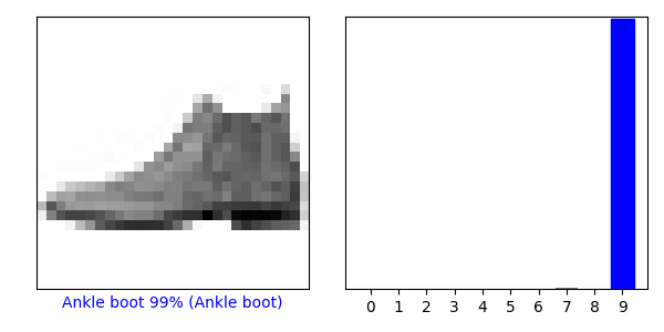
i = 0
plt.figure(figsize=(6, 3))
plt.subplot(1, 2, 1)
plot_image(i, predictions[i], test_labels, test_images)
plt.subplot(1, 2, 2)
plot_value_array(i, predictions[i], test_labels)
plt.show()
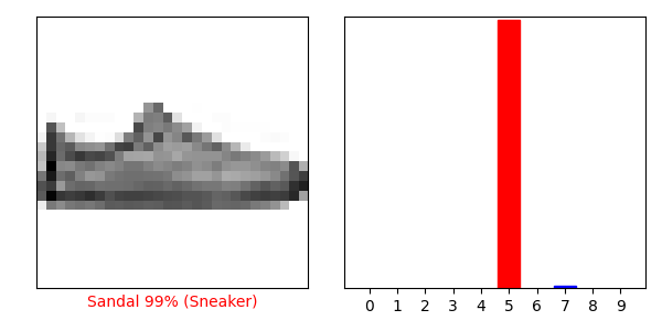
i = 12
plt.figure(figsize=(6, 3))
plt.subplot(1, 2, 1)
plot_image(i, predictions[i], test_labels, test_images)
plt.subplot(1, 2, 2)
plot_value_array(i, predictions[i], test_labels)
plt.show()
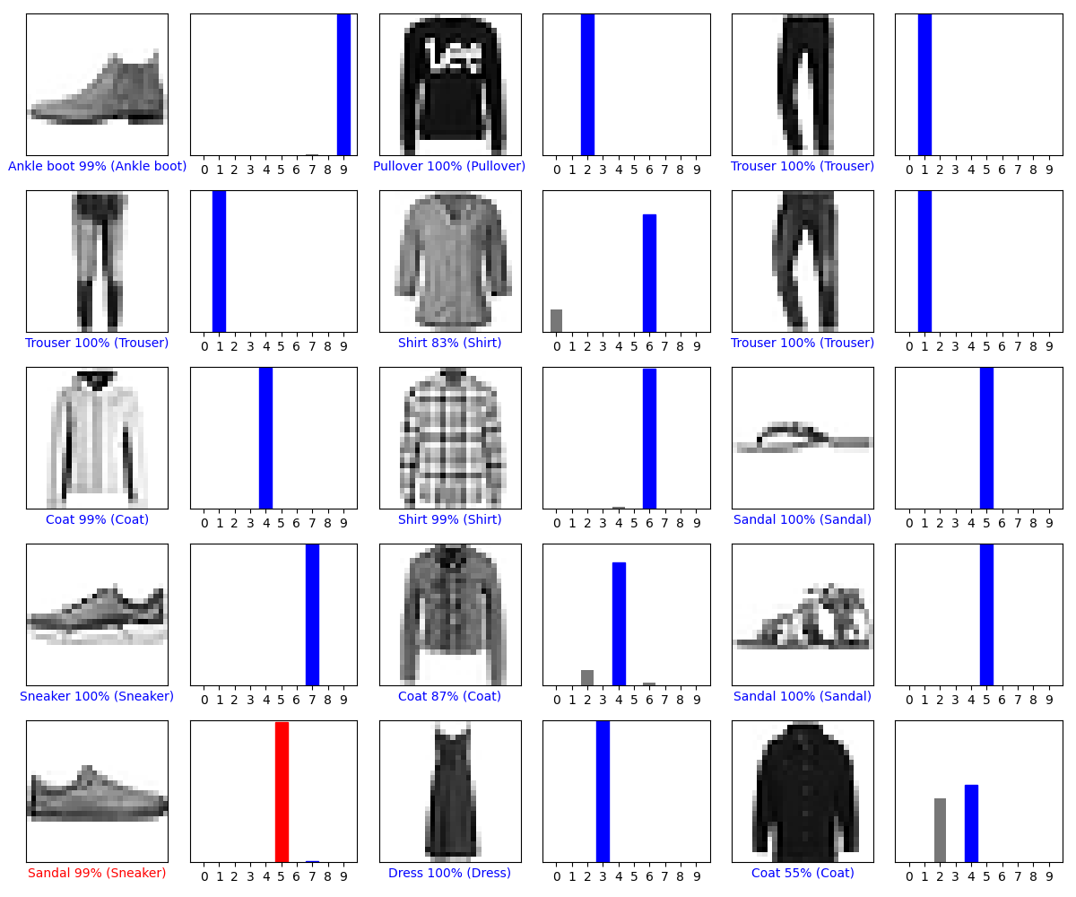
# Plot the first X test images, their predicted labels, and the true labels.
# Color correct predictions in blue and incorrect predictions in red.
num_rows = 5
num_cols = 3
num_images = num_rows * num_cols
plt.figure(figsize=(2 * 2 * num_cols, 2 * num_rows))
for i in range(num_images):
plt.subplot(num_rows, 2 * num_cols, 2 * i + 1)
plot_image(i, predictions[i], test_labels, test_images)
plt.subplot(num_rows, 2 * num_cols, 2 * i + 2)
plot_value_array(i, predictions[i], test_labels)
plt.tight_layout()
plt.show()
# Grab an image from the test dataset.
img = test_images[1]
print(img.shape)
# Add the image to a batch where it's the only member.
img = (np.expand_dims(img, 0))
print(img.shape)
predictions_single = probability_model.predict(img)
print(predictions_single)
plot_value_array(1, predictions_single[0], test_labels)
_ = plt.xticks(range(10), class_names, rotation=45)
np.argmax(predictions_single[0])
结果:
Epoch 1/10
1875/1875 [==============================] - 1s 468us/step - loss: 0.4987 - accuracy: 0.8241
Epoch 2/10
1875/1875 [==============================] - 1s 468us/step - loss: 0.3763 - accuracy: 0.8647
Epoch 3/10
1875/1875 [==============================] - 1s 476us/step - loss: 0.3372 - accuracy: 0.8771
Epoch 4/10
1875/1875 [==============================] - 1s 468us/step - loss: 0.3118 - accuracy: 0.8855
Epoch 5/10
1875/1875 [==============================] - 1s 467us/step - loss: 0.2950 - accuracy: 0.8913
Epoch 6/10
1875/1875 [==============================] - 1s 464us/step - loss: 0.2808 - accuracy: 0.8957
Epoch 7/10
1875/1875 [==============================] - 1s 458us/step - loss: 0.2677 - accuracy: 0.9008
Epoch 8/10
1875/1875 [==============================] - 1s 461us/step - loss: 0.2588 - accuracy: 0.9049
Epoch 9/10
1875/1875 [==============================] - 1s 461us/step - loss: 0.2485 - accuracy: 0.9079
Epoch 10/10
1875/1875 [==============================] - 1s 462us/step - loss: 0.2395 - accuracy: 0.9099
313/313 - 0s - loss: 0.3524 - accuracy: 0.8790
Test accuracy: 0.8790000081062317
(28, 28)
(1, 28, 28)
[[2.8769002e-05 4.6691982e-16 9.9956042e-01 3.8130179e-09 2.9655307e-04
  2.2426191e-12 1.1432933e-04 1.4692046e-18 1.0452014e-11 1.5957140e-17]]
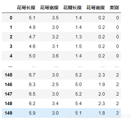
2.鸢尾花分类问题
#导入相关包
from sklearn.datasets import load_iris#导入数据集
from pandas import DataFrame
import pandas as pd


x_data=load_iris().data #返回iris数据集的所有输入
y_data=load_iris().target  #返回iris数据集中所有标签


x_data=DataFrame(x_data,columns=['花萼长度','花萼宽度','花瓣长度','花萼宽度'])
pd.set_option('display.unicode.east_asian_width',True) #设置列名对其

x_data['类别']=y_data #添加一列,列标签为列表
# 导入所需模块
import tensorflow as tf
from sklearn import datasets
from matplotlib import pyplot as plt
%matplotlib inline
import numpy as np
# 导入数据,分别为输入特征和标签
x_data = datasets.load_iris().data
y_data = datasets.load_iris().target
# 随机打乱数据(因为原始数据是顺序的,顺序不打乱会影响准确率)
# seed: 随机数种子,是一个整数,当设置之后,每次生成的随机数都一样(为方便教学,以保每位同学结果一致)
np.random.seed(116) # 使用相同的seed,保证输入特征和标签一一对应
np.random.shuffle(x_data)
np.random.seed(116)
np.random.shuffle(y_data)
tf.random.set_seed(116)
# 将打乱后的数据集分割为训练集和测试集,训练集为前120行,测试集为后30行
x_train = x_data[:-30]
y_train = y_data[:-30]
x_test = x_data[-30:]
y_test = y_data[-30:]
# 转换x的数据类型,否则后面矩阵相乘时会因数据类型不一致报错
x_train = tf.cast(x_train, tf.float32)
x_test = tf.cast(x_test, tf.float32)
# from_tensor_slices函数使输入特征和标签值一一对应。(把数据集分批次,每个批次batch组数据)
train_db = tf.data.Dataset.from_tensor_slices((x_train, y_train)).batch(32)
test_db = tf.data.Dataset.from_tensor_slices((x_test, y_test)).batch(32)
# 生成神经网络的参数,4个输入特征故,输入层为4个输入节点;因为3分类,故输出层为3个神经元
# 用tf.Variable()标记参数可训练
# 使用seed使每次生成的随机数相同(方便教学,使大家结果都一致,在现实使用时不写seed)
w1 = tf.Variable(tf.random.truncated_normal([4, 3], stddev=0.1, seed=1))
b1 = tf.Variable(tf.random.truncated_normal([3], stddev=0.1, seed=1))
#定义超参数
lr = 0.1 # 学习率为0.1
train_loss_results = [] # 将每轮的loss记录在此列表中,为后续画loss曲线提供数据
test_acc = [] # 将每轮的acc记录在此列表中,为后续画acc曲线提供数据
epoch = 500 # 循环500轮
loss_all = 0 # 每轮分4个step,loss_all记录四个step生成的4个loss的和
# 训练部分
for epoch in range(epoch): #数据集级别的循环,每个epoch循环一次数据集
for step, (x_train, y_train) in enumerate(train_db): #batch级别的循环 ,每个step循环一个batch
with tf.GradientTape() as tape: # with结构记录梯度信息
y = tf.matmul(x_train, w1) + b1 # 神经网络乘加运算
y = tf.nn.softmax(y) # 使输出y符合概率分布(此操作后与独热码同量级,可相减求loss)
y_ = tf.one_hot(y_train, depth=3) # 将标签值转换为独热码格式,方便计算loss和accuracy
loss = tf.reduce_mean(tf.square(y_ - y)) # 采用均方误差损失函数mse = mean(sum(y-out)^2)
loss_all += loss.numpy() # 将每个step计算出的loss累加,为后续求loss平均值提供数据,这样计算的loss更准确
# 计算loss对各个参数的梯度
grads = tape.gradient(loss, [w1, b1])
# 实现梯度更新 w1 = w1 - lr * w1_grad b = b - lr * b_grad
w1.assign_sub(lr * grads[0]) # 参数w1自更新
b1.assign_sub(lr * grads[1]) # 参数b自更新
# 每个epoch,打印loss信息
print("Epoch {}, loss: {}".format(epoch, loss_all/4))
train_loss_results.append(loss_all / 4) # 将4个step的loss求平均记录在此变量中
loss_all = 0 # loss_all归零,为记录下一个epoch的loss做准备
# 测试部分
# total_correct为预测对的样本个数, total_number为测试的总样本数,将这两个变量都初始化为0
total_correct, total_number = 0, 0
for x_test, y_test in test_db:
# 使用更新后的参数进行预测
y = tf.matmul(x_test, w1) + b1#计算前向传播预测结果
y = tf.nn.softmax(y)#变为概率分布
pred = tf.argmax(y, axis=1) # 返回y中最大值的索引,即预测的分类
# 将pred转换为y_test的数据类型
pred = tf.cast(pred, dtype=y_test.dtype)
# 若分类正确,则correct=1,否则为0,将bool型的结果转换为int型
correct = tf.cast(tf.equal(pred, y_test), dtype=tf.int32)
# 将每个batch的correct数加起来
correct = tf.reduce_sum(correct)
# 将所有batch中的correct数加起来
total_correct += int(correct)
# total_number为测试的总样本数,也就是x_test的行数,shape[0]返回变量的行数
total_number += x_test.shape[0]
# 总的准确率等于total_correct/total_number
acc = total_correct / total_number
test_acc.append(acc)
print("Test_acc:", acc)
print("--------------------------")
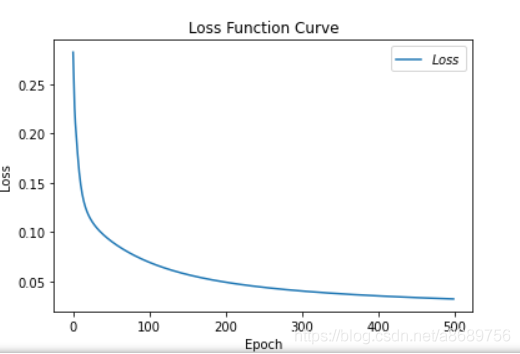
# 绘制 loss 曲线
plt.title('Loss Function Curve') # 图片标题
plt.xlabel('Epoch') # x轴变量名称
plt.ylabel('Loss') # y轴变量名称
plt.plot(train_loss_results, label="$Loss$") # 逐点画出trian_loss_results值并连线,连线图标是Loss
plt.legend() # 画出曲线图标
plt.show() # 画出图像
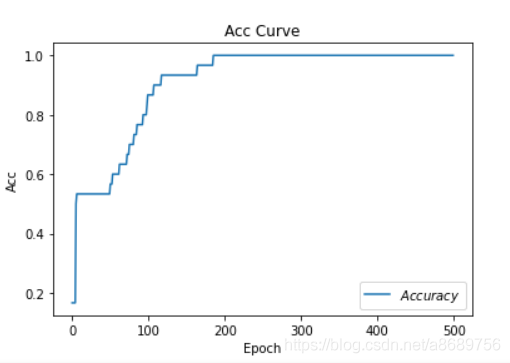
# 绘制 Accuracy 曲线
plt.title('Acc Curve') # 图片标题
plt.xlabel('Epoch') # x轴变量名称
plt.ylabel('Acc') # y轴变量名称
plt.plot(test_acc, label="$Accuracy$") # 逐点画出test_acc值并连线,连线图标是Accuracy
plt.legend()
plt.show()

 浙公网安备 33010602011771号