浅谈压缩感知(二十六):压缩感知重构算法之分段弱正交匹配追踪(SWOMP)
主要内容:
- SWOMP的算法流程
- SWOMP的MATLAB实现
- 一维信号的实验与结果
- 门限参数a、测量数M与重构成功概率关系的实验与结果
- SWOMP与StOMP性能比较
一、SWOMP的算法流程
分段弱正交匹配追踪(Stagewise Weak OMP)可以说是StOMP的一种修改算法,它们的唯一不同是选择原子时的门限设置,这可以降低对测量矩阵的要求。我们称这里的原子选择方式为"弱选择"(Weak Selection),StOMP的门限设置由残差决定,这对测量矩阵(原子选择)提出了要求,而SWOMP的门限设置则对测量矩阵要求较低(原子选择相对简单、粗糙)。
SWOMP的算法流程:
二、SWOMP的MATLAB实现(CS_SWOMP.m)
function [ theta ] = CS_SWOMP( y,A,S,alpha )
%   CS_SWOMP
%   Detailed explanation goes here
%   y = Phi * x
%   x = Psi * theta
%    y = Phi*Psi * theta
%   令 A = Phi*Psi, 则y=A*theta
%   S is the maximum number of SWOMP iterations to perform
%   alpha is the threshold parameter
%   现在已知y和A,求theta
%   Reference:Thomas Blumensath,Mike E. Davies.Stagewise weak gradient
%   pursuits[J].IEEE Transactions on Signal Processing,2009,57(11):4333-4346.
    if nargin < 4
        alpha = 0.5; %alpha范围(0,1),默认值为0.5
    end
    if nargin < 3
        S = 10; %S默认值为10
    end
    [y_rows,y_columns] = size(y);
    if y_rows<y_columns
        y = y'; %y should be a column vector
    end
    [M,N] = size(A); %传感矩阵A为M*N矩阵
    theta = zeros(N,1); %用来存储恢复的theta(列向量)
    Pos_theta = []; %用来迭代过程中存储A被选择的列序号
    r_n = y; %初始化残差(residual)为y
    for ss=1:S %最多迭代S次
        product = A'*r_n; %传感矩阵A各列与残差的内积
        sigma = max(abs(product));
        Js = find(abs(product)>=alpha*sigma); %选出大于阈值的列
        Is = union(Pos_theta,Js); %Pos_theta与Js并集
        if length(Pos_theta) == length(Is)
            if ss==1
                theta_ls = 0; %防止第1次就跳出导致theta_ls无定义
            end
            break; %如果没有新的列被选中则跳出循环
        end
        %At的行数要大于列数,此为最小二乘的基础(列线性无关)
        if length(Is)<=M
            Pos_theta = Is; %更新列序号集合
            At = A(:,Pos_theta); %将A的这几列组成矩阵At
        else%At的列数大于行数,列必为线性相关的,At'*At将不可逆
            if ss==1
                theta_ls = 0; %防止第1次就跳出导致theta_ls无定义
            end
            break; %跳出for循环
        end
        %y=At*theta,以下求theta的最小二乘解(Least Square)
        theta_ls = (At'*At)^(-1)*At'*y; %最小二乘解
        %At*theta_ls是y在At列空间上的正交投影
        r_n = y - At*theta_ls; %更新残差
        if norm(r_n)<1e-6 %Repeat the steps until r=0
            break; %跳出for循环
        end
    end
    theta(Pos_theta)=theta_ls;%恢复出的theta
end
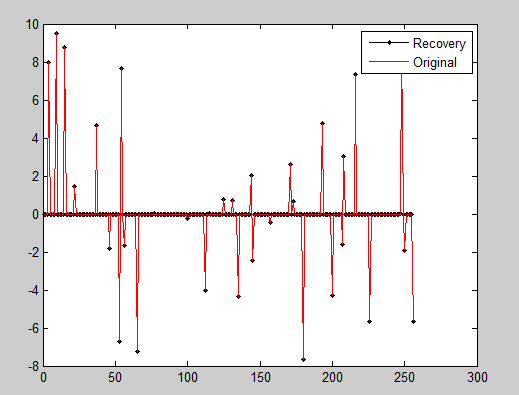
三、一维信号的实验与结果
%压缩感知重构算法测试
clear all;close all;clc;
M = 128; %观测值个数
N = 256; %信号x的长度
K = 30; %信号x的稀疏度
Index_K = randperm(N);
x = zeros(N,1);
x(Index_K(1:K)) = 5*randn(K,1); %x为K稀疏的,且位置是随机的
Psi = eye(N); %x本身是稀疏的,定义稀疏矩阵为单位阵x=Psi*theta
Phi = randn(M,N)/sqrt(M); %测量矩阵为高斯矩阵
A = Phi * Psi; %传感矩阵
y = Phi * x; %得到观测向量y

%% 恢复重构信号x
tic
theta = CS_SWOMP( y,A);
x_r = Psi * theta; % x=Psi * theta
toc

%% 绘图
figure;
plot(x_r,'k.-'); %绘出x的恢复信号
hold on;
plot(x,'r'); %绘出原信号x
hold off;
legend('Recovery','Original')
fprintf('\n恢复残差:');
norm(x_r-x) %恢复残差
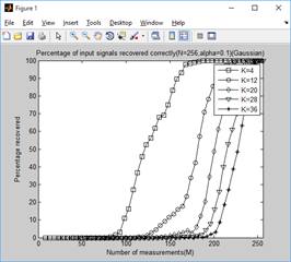
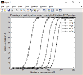
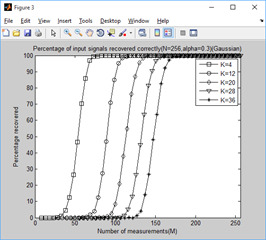
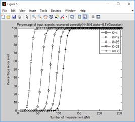
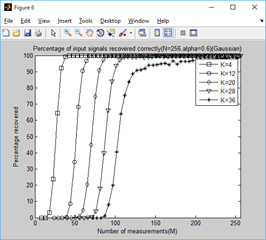
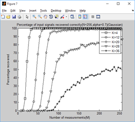
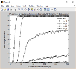
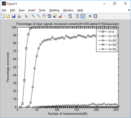
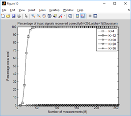
四、门限参数a、测量数M与重构成功概率关系的实验与结果
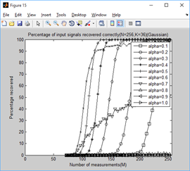
1、门限参数a分别为0.1-1.0时,不同稀疏信号下,测量值M与重构成功概率的关系:
clear all;close all;clc;

%% 参数配置初始化
CNT = 1000; %对于每组(K,M,N),重复迭代次数
N = 256; %信号x的长度
Psi = eye(N); %x本身是稀疏的,定义稀疏矩阵为单位阵x=Psi*theta
alpha_set = 0.1:0.1:1;
K_set = [4,12,20,28,36]; %信号x的稀疏度集合
Percentage = zeros(N,length(K_set),length(alpha_set)); %存储恢复成功概率

%% 主循环,遍历每组(alpha,K,M,N)
tic
for tt = 1:length(alpha_set)
    alpha = alpha_set(tt);
    for kk = 1:length(K_set)
        K = K_set(kk); %本次稀疏度
        %M没必要全部遍历,每隔5测试一个就可以了
        M_set=2*K:5:N;
        PercentageK = zeros(1,length(M_set)); %存储此稀疏度K下不同M的恢复成功概率
        for mm = 1:length(M_set)
           M = M_set(mm); %本次观测值个数
           fprintf('alpha=%f,K=%d,M=%d\n',alpha,K,M);
           P = 0;
           for cnt = 1:CNT  %每个观测值个数均运行CNT次
                Index_K = randperm(N);
                x = zeros(N,1);
                x(Index_K(1:K)) = 5*randn(K,1); %x为K稀疏的,且位置是随机的
                Phi = randn(M,N)/sqrt(M); %测量矩阵为高斯矩阵
                A = Phi * Psi; %传感矩阵
                y = Phi * x; %得到观测向量y
                theta = CS_SWOMP(y,A,10,alpha); %恢复重构信号theta
                x_r = Psi * theta; % x=Psi * theta
                if norm(x_r-x)<1e-6 %如果残差小于1e-6则认为恢复成功
                    P = P + 1;
                end
           end
           PercentageK(mm) = P/CNT*100; %计算恢复概率
        end
        Percentage(1:length(M_set),kk,tt) = PercentageK;
    end
end
toc
save SWOMPMtoPercentage1000 %运行一次不容易,把变量全部存储下来

%% 绘图
for tt = 1:length(alpha_set)
    S = ['-ks';'-ko';'-kd';'-kv';'-k*'];
    figure;
    for kk = 1:length(K_set)
        K = K_set(kk);
        M_set=2*K:5:N;
        L_Mset = length(M_set);
        plot(M_set,Percentage(1:L_Mset,kk,tt),S(kk,:));%绘出x的恢复信号
        hold on;
    end
    hold off;
    xlim([0 256]);
    legend('K=4','K=12','K=20','K=28','K=36');
    xlabel('Number of measurements(M)');
    ylabel('Percentage recovered');
    title(['Percentage of input signals recovered correctly(N=256,alpha=',...
        num2str(alpha_set(tt)),')(Gaussian)']);
end
for kk = 1:length(K_set)
    K = K_set(kk);
    M_set=2*K:5:N;
    L_Mset = length(M_set);
    S = ['-ks';'-ko';'-kd';'-k*';'-k+';'-kx';'-kv';'-k^';'-k<';'-k>'];
    figure;
    for tt = 1:length(alpha_set)
        plot(M_set,Percentage(1:L_Mset,kk,tt),S(tt,:));%绘出x的恢复信号
        hold on;
    end
    hold off;
    xlim([0 256]);
    legend('alpha=0.1','alpha=0.2','alpha=0.3','alpha=0.4','alpha=0.5',...
        'alpha=0.6','alpha=0.7','alpha=0.8','alpha=0.9','alpha=1.0');
    xlabel('Number of measurements(M)');
    ylabel('Percentage recovered');
    title(['Percentage of input signals recovered correctly(N=256,K=',...
        num2str(K),')(Gaussian)']);
end

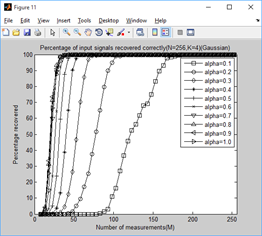
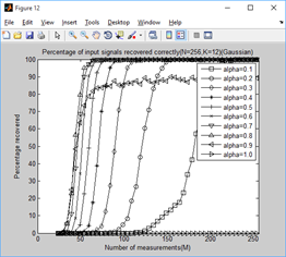
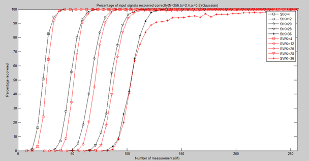
2、稀疏度为4,12,20,28,36时,不同门限参数a下,测量值M与重构成功概率的关系:
clear all;close all;clc;
load StOMPMtoPercentage1000;
PercentageStOMP = Percentage;
S = ['-ks';'-ko';'-kd';'-kv';'-k*'];
figure;
for kk = 1:length(K_set)
    K = K_set(kk);
    M_set=2*K:5:N;
    L_Mset = length(M_set);
    %ts_set = 2:0.2:3;第3个为2.4
    plot(M_set,Percentage(1:L_Mset,kk,3),S(kk,:));%绘出x的恢复信号
    hold on;
end
load SWOMPMtoPercentage1000;
PercentageSWOMP = Percentage;
S = ['-rs';'-ro';'-rd';'-rv';'-r*'];
for kk = 1:length(K_set)
    K = K_set(kk);
    M_set=2*K:5:N;
    L_Mset = length(M_set);
    %alpha_set = 0.1:0.1:1;第6个为0.6
    plot(M_set,Percentage(1:L_Mset,kk,6),S(kk,:));%绘出x的恢复信号
    hold on;
end
hold off;
xlim([0 256]);
legend('StK=4','StK=12','StK=20','StK=28','StK=36',...
    'SWK=4','SWK=12','SWK=20','SWK=28','SWK=36');
xlabel('Number of measurements(M)');
ylabel('Percentage recovered');
title(['Percentage of input signals recovered correctly(N=256,ts=2.4,\alpha=0.5)(Gaussian)']);
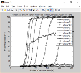
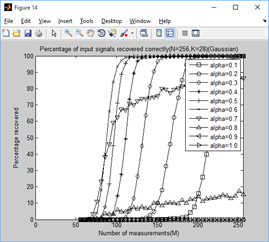
结论:
通过对比可以看出,总体上讲a=0.6时效果较好。
五、SWOMP与StOMP性能比较
对比StOMP中ts=2.4与SWOMP中α=0.6的情况:StOMP要略好于SWOMP。

 浙公网安备 33010602011771号