通过线性回归来理解pytorch的计算逻辑

 

首先，声明本文非原创，参考博客：https://shartoo.github.io/2019/10/28/-understand-pytorch/

只是想自己记录一下，更好的理解pytorch的计算。

1、线性回归问题

假定我们以一个线性回归问题来逐步解释pytorch过程中的一些操作和逻辑。线性回归公式如下：

1.1 先用普通的numpy来展示线性回归过程

随机生成100个数据，并以一定的随机概率扰动数据集，训练集和验证集八二分，如下：

# 数据生成
np.random.seed(42)
x = np.random.rand(100, 1)
y = 1 + 2 * x + .1 * np.random.randn(100, 1)

# Shuffles the indices
idx = np.arange(100)
np.random.shuffle(idx)

# Uses first 80 random indices for train
train_idx = idx[:80]
# Uses the remaining indices for validation
val_idx = idx[80:]

# Generates train and validation sets
x_train, y_train = x[train_idx], y[train_idx]
x_val, y_val = x[val_idx], y[val_idx]

上面这是我们已经知道的是一个线性回归数据分布，并且回归的参数是a=1,b=2  如果我们只知道数据x_train和y_train，需要求这两个参数a,b呢，一般是使用梯度下降方法。

注意，下面的梯度下降方法是全量梯度，一次计算了所有的数据的梯度，只是在迭代了1000个epoch，通常训练时会把全量数据分成多个batch，每次都是小批量更新。

# 初始化线性回归的参数 a 和 b
np.random.seed(42)
a = np.random.randn(1)
b = np.random.randn(1)
print("初始化的 a : %d 和 b : %d"%(a,b))
leraning_rate = 1e-2
epochs = 1000
for epoch in range(epochs):
    pred = a+ b*x_train
    # 计算预测值和真实值之间的误差
    error = y_train-pred
    # 使用MSE 来计算回归误差
    loss = (error**2).mean()
    # 计算参数 a 和 b的梯度
    a_grad = -2*error.mean()
    b_grad = -2*(x_train*error).mean()
    # 更新参数：用学习率和梯度
    a = a-leraning_rate*a_grad
    b = b -leraning_rate*b_grad

print("最终获得参数为 a : %.2f, b :%.2f "%(a,b))

得到的输出如下：

初始化的 a : 0 和 b : 0
最终获得参数为 a : 0.98, b :1.94

2 pytorhc 来解决回归问题

2.1 pytorch的一些基础问题

• 如果将numpy数组转化为pytorch的tensor呢？使用torch.from_numpy(data)
• 如果想将计算的数据放入GPU计算：data.to(device)(其中的device就是GPU或cpu)
• 数据类型转换示例： data.float()
• 如果确定数据位于CPU还是GPU:data.type()会得到类似于torch.cuda.FloatTensor的结果，表明在GPU中
• 从GPU中把数据转化成numpy：先取出到cpu中，再转化成numpy数组。data.cpu().numpy()

2.2 使用pytorch构建参数

如何区分普通数据和参数/权重呢？需要计算梯度的是参数，否则就是普通数据。参数需要用梯度来更新，我们需要选项requires_grad=True。使用了这个选项就是告诉pytorch，我们要计算此变量的梯度了。

我们可以使用如下几种方式来构建参数：

1、此方法构建出来的参数全部都在cpu中：

a = torch.randn(1, requires_grad=True, dtype=torch.float)
b = torch.randn(1, requires_grad=True, dtype=torch.float)
print(a, b)

2、此方法尝试把tensor参数传入到gpu：

a = torch.randn(1, requires_grad=True, dtype=torch.float).to(device)
b = torch.randn(1, requires_grad=True, dtype=torch.float).to(device)
print(a, b)

此时如果查看输出，会发现两个tensor ，a和b的梯度选项没了（没了requires_grad=True）

tensor([0.5158], device='cuda:0', grad_fn=<CopyBackwards>) tensor([0.0246], device='cuda:0', grad_fn=<CopyBackwards>)

3、先将tensor传入gpu，然后再使用requires_grad_()选项来重构tensor的属性。

a = torch.randn(1, dtype=torch.float).to(device)
b = torch.randn(1, dtype=torch.float).to(device)
# and THEN set them as requiring gradients...
a.requires_grad_()
b.requires_grad_()
print(a, b)

4、最佳策略当然是初始化的时候直接赋予requires_grad=True属性了

 

# We can specify the device at the moment of creation - RECOMMENDED!
torch.manual_seed(42)
a = torch.randn(1, requires_grad=True, dtype=torch.float, device=device)
b = torch.randn(1, requires_grad=True, dtype=torch.float, device=device)
print(a, b)

 

查看tensor属性：

tensor([0.6226], device='cuda:0', requires_grad=True) tensor([1.4505], device='cuda:0', requires_grad=True)

2.3 自动求导 Autograd

Autograd是Pytorch的自动求导包，有了它，我们就不必担忧偏导数和链式法则等一系列问题。Pytorch计算所有梯度的方法是backward()。计算梯度之前，我们需要先计算损失，那么需要调用对应(损失)变量的求导方法，如loss.backward()。

• 计算所有变量的梯度(假设损失变量是loss): loss.back()
• 获取某个变量的实际的梯度值(假设变量为att):att.grad
• 由于梯度是累加的，每次用梯度更新参数之后，需要清零(假设梯度变量是att):att.zero_(),下划线是一种运算符，相当于直接作用于原变量上，等同于att=0(不要手动赋值，因为此过程可能涉及到GPU、CPU之间数据传输，容易出错)

我们接下来尝试下手工更新参数和梯度

 

lr = 1e-1
n_epochs = 1000

torch.manual_seed(42)
a = torch.randn(1, requires_grad=True, dtype=torch.float, device=device)
b = torch.randn(1, requires_grad=True, dtype=torch.float, device=device)

for epoch in range(n_epochs):
    yhat = a + b * x_train_tensor
    error = y_train_tensor - yhat
    loss = (error ** 2).mean()

    # 这个是numpy的计算梯度的方式
    # a_grad = -2 * error.mean()
    # b_grad = -2 * (x_tensor * error).mean()
    
    # 告诉pytorch计算损失loss，计算所有变量的梯度
    loss.backward()
    # 打印结果
    print(a.grad)
    print(b.grad)  
    
    # 1. 手动更新参数，会出错 AttributeError: 'NoneType' object has no attribute 'zero_'
    # 错误的原因是，我们重新赋值时会丢掉变量的 梯度属性
    # a = a - lr * a.grad
    # b = b - lr * b.grad
    # print(a)
    # 2. 再次手动更新参数，这次我们没有重新赋值，而是使用in-place的方式赋值  RuntimeError: a leaf Variable that requires grad has been used in an in- place operation.
    # 这是因为 pytorch 给所有需要计算梯度的python操作以及依赖都纳入了动态计算图，稍后会解释
    # a -= lr * a.grad
    # b -= lr * b.grad        

    # 3. 如果我们真想手动更新，不使用pytorch的计算图呢，必须使用no_grad来将此参数移除自动计算梯度变量之外。
    # 这是源于pytorch的动态计算图DYNAMIC GRAPH，后面会有详细的解释
    with torch.no_grad():
        a -= lr * a.grad
        b -= lr * b.grad
    
    # PyTorch is "clingy" to its computed gradients, we need to tell it to let it go...
    a.grad.zero_()
    b.grad.zero_()
    
print(a, b)

 

2.4 动态计算图

如果想可视化计算图，可以使用辅助包torchviz，需要自己安装。使用其make_dot(变量)方法来可视化与当前给定变量相关的计算图。示例

 

torch.manual_seed(42)
a = torch.randn(1, requires_grad=True, dtype=torch.float, device=device)
b = torch.randn(1, requires_grad=True, dtype=torch.float, device=device)

yhat = a + b * x_train_tensor
error = y_train_tensor - yhat
loss = (error ** 2).mean()
make_dot(yhat)

 

使用make_dot(yhat)会得到相关的三个计算图如下：

 

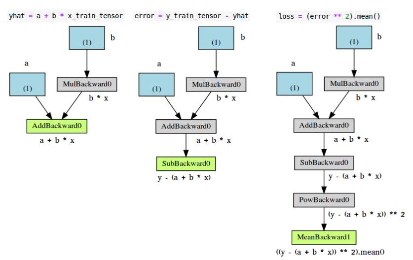
各个组件，解释如下

 

• 蓝色盒子：作为参数的tensor，需要pytorch计算梯度的
• 灰色盒子：与计算梯度相关的或者计算梯度依赖的，python操作
• 绿色盒子：与灰色盒子一样，区别是，它是计算梯度的起始点（假设backward()方法是需要可视化图的变量调用的）-计算图自底向上构建。

 

上图的error(图中)和loss(图右)，与左图的唯一区别就是中间步骤(灰色盒子)的数目。看左边的绿色盒子，有两个箭头指向该绿色盒子，代表两个变量相加。a和b*x。再看该图中的灰色盒子，它执行的是乘法计算，即b*x，但是为啥只有一个箭头指向呢，只有来自蓝色盒子的参数b，为啥没有数据x?因为我们不需要为数据x计算梯度（不计算梯度的变量不会出现在计算图中）。那么，如果我们去掉变量的requires_grad属性(设置为False)会怎样？

 

a_nongrad = torch.randn(1,requires_grad=False,dtype=torch.float,device=device)
b = torch.randn(1,requires_grad=True,dtype=torch.float,device=device)
yhat = a_nongrad+b*x_train_tensor

 

 

 

 

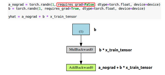
可以看到，对应参数a的蓝色盒子没有了，所以很简单明了，不计算梯度，就不出现在计算图中。

 

3 优化器 Optimizer

 

到目前为止，我们都是手动计算梯度并更新参数的，如果有非常多的变量。我们可以使用pytorch的优化器，像SGD或者Adam。

 

优化器需要指定需要优化的参数，以及学习率，然后使用step()方法来更新，此外，我们不必再一个个的去将梯度赋值为0了，只需要使用优化器的zero_grad()方法即可。。

 

代码示例，使用SGD优化器更新参数a和b的梯度。

torch.manual_seed(42)
a = torch.randn(1, requires_grad=True, dtype=torch.float, device=device)
b = torch.randn(1, requires_grad=True, dtype=torch.float, device=device)
print(a, b)

lr = 1e-1
n_epochs = 1000

# Defines a SGD optimizer to update the parameters
optimizer = optim.SGD([a, b], lr=lr)

for epoch in range(n_epochs):
    # 第一步，计算损失
    yhat = a + b * x_train_tensor
    error = y_train_tensor - yhat
    loss = (error ** 2).mean()
    # 第二步，后传损失
    loss.backward()    
    
    # 不用再手动更新参数了
    # with torch.no_grad():
    # a -= lr * a.grad
    # b -= lr * b.grad
    # 使用优化器的step方法一步到位
    optimizer.step()
    
    # 也不用告诉pytorch需要对哪些梯度清零操作了，优化器的zero_grad()一步到位
    # a.grad.zero_()
    # b.grad.zero_()
    optimizer.zero_grad()
    
print(a, b)

4 计算损失loss

pytorch提供了很多损失函数，可以直接调用。简单使用如下：

torch.manual_seed(42)
a = torch.randn(1, requires_grad=True, dtype=torch.float, device=device)
b = torch.randn(1, requires_grad=True, dtype=torch.float, device=device)
print(a, b)

lr = 1e-1
n_epochs = 1000

# 此处定义了损失函数为MSE
loss_fn = nn.MSELoss(reduction='mean')

optimizer = optim.SGD([a, b], lr=lr)

for epoch in range(n_epochs):
    yhat = a + b * x_train_tensor
    
    # 不用再手动计算损失了
    # error = y_tensor - yhat
    # loss = (error ** 2).mean()
    # 直接调用定义好的损失函数即可
    loss = loss_fn(y_train_tensor, yhat)

    loss.backward()    
    optimizer.step()
    optimizer.zero_grad()
    
print(a, b)

5 模型

pytorch中模型由一个继承自Module的Python类来定义。需要实现两个最基本的方法

1. __init__(self):定义了模型由哪几部分组成，当前模型只有两个变量a和b。模型可以定义更多的参数，并且可以将其他模型或者网络层定义为其参数
2. forwad(self,x):真实执行计算的方法，它对给定输入x输出模型预测值。不要显示调用此forward(x)方法，而是直接调用模型本身，即model(x)。

简单的回归模型如下：

class ManualLinearRegression(nn.Module):
    def __init__(self):
        super().__init__()
        # To make "a" and "b" real parameters of the model, we need to wrap them with nn.Parameter
        self.a = nn.Parameter(torch.randn(1, requires_grad=True, dtype=torch.float))
        self.b = nn.Parameter(torch.randn(1, requires_grad=True, dtype=torch.float))
        
    def forward(self, x):
        # 计算预测结果
        return self.a + self.b * x

在__init__(self)方法中，我们使用Parameters()类定义了两个参数a和b，告诉Pytorch，这两个tensor要被作为模型的参数的属性。这样，我们就可以使用模型的parameters()方法来找到模型每次迭代时的所有参数值了，即便模型是嵌套模型都可以找得到，这样就能将参数喂入优化器optimizer来计算了(而非手动维护一张参数表)。并且，我们可以使用模型的state_dict()方法来获取所有参数的当前值。

注意：模型应当与数据出于相同位置(GPU/CPU)，如果数据时GPU tensor，我们的模型也必须在GPU中

代码示例如下:

torch.manual_seed(42)

# Now we can create a model and send it at once to the device
model = ManualLinearRegression().to(device)
# 获取所有参数的当前值
print(model.state_dict())

lr = 1e-1
n_epochs = 1000

loss_fn = nn.MSELoss(reduction='mean')
optimizer = optim.SGD(model.parameters(), lr=lr)

for epoch in range(n_epochs):
    #  注意，模型一般都有个train()方法，但是不要手动调用，此处只是为了说明此时是在训练，防止有些模型在训练模型和验证模型时操作不一致，训练时有dropout之类的
    model.train()

    # yhat = a + b * x_tensor
    yhat = model(x_train_tensor)
    
    loss = loss_fn(y_train_tensor, yhat)
    loss.backward()    
    optimizer.step()
    optimizer.zero_grad()
    
print(model.state_dict())

6 训练

我们定义了optimizer,loss function,model为模型三要素，同时需要提供训练时用的特征(feature)和对应的标签(label)数据。一个完整的模型训练有以下组成

• 模型三要素
  • 优化器optimizer
  • 损失函数loss
  • 模型 model
• 数据
  • 特征数据feature
  • 数据标签label

我们可以写一个包含模型三要素的通用的训练函数：

def make_train_step(model, loss_fn, optimizer):
    # 定义一个训练函数
    def train_step(x, y):
        # Sets model to TRAIN mode
        model.train()
        # 模型预测
        yhat = model(x)
        # 计算损失
        loss = loss_fn(y, yhat)
        # 计算梯度
        loss.backward()
        # 更新参数以及梯度清零
        optimizer.step()
　　　　
        optimizer.zero_grad()
        # Returns the loss
        return loss.item()
    
    # Returns the function that will be called inside the train loop
    return train_step

然后在每个epoch时迭代模型训练

# Creates the train_step function for our model, loss function and optimizer
train_step = make_train_step(model, loss_fn, optimizer)
losses = []

# For each epoch...
for epoch in range(n_epochs):
    # Performs one train step and returns the corresponding loss
    loss = train_step(x_train_tensor, y_train_tensor)
    losses.append(loss)
    
# Checks model's parameters
print(model.state_dict())

 最后梳理一下pytorch计算的整个流程：

1、创建线性回归的模型类；

2、创建数据；

3、训练调用模型进行预测；

4、计算损失（预先定义损失函数）；

5、optimizer.zero_grad() 清空过往梯度；

6、loss.backward() 反向传播，计算当前梯度；

7、optimizer.step() 根据梯度更新网络参数；

8、保存模型；

 

最后，附上一个完整的线性回归训练及预测模型的代码：

#!D:/CODE/python
# -*- coding: utf-8 -*-
# @Time : 2020/8/11 19:02
# @Author : Alex-bd
# @Site :
# @File : pytorch计算逻辑.py
# @Software: PyCharm
# Functional description:通过线性回归学习pytorch计算逻辑

import os
os.environ['KMP_DUPLICATE_LIB_OK'] = 'TRUE'
import torch
import matplotlib.pyplot as plt


def create_linear_data(nums_data, if_plot=False):
    """
    Create data for linear model
    Args:
        nums_data: how many data points that wanted
    Returns:
        x with shape (nums_data, 1)
    """
    x = torch.linspace(0, 1, nums_data)
    x = torch.unsqueeze(x, dim=1)
    b = 3
    a = 1
    y = a + b * x + torch.rand(x.size())

    if if_plot:
        plt.scatter(x.numpy(), y.numpy(), c=x.numpy())
        plt.show()
    data = {"x": x, "y": y}
    return data


data = create_linear_data(300, if_plot=True)
print(data["x"].size())


class LinearRegression(torch.nn.Module):
    """
    Linear Regressoin Module, the input features and output
    features are defaults both 1
    """

    def __init__(self):
        super().__init__()
        # self.linear = torch.nn.Linear(1, 1)
        self.a = torch.nn.Parameter(torch.randn(1, requires_grad=True, dtype=torch.float))
        self.b = torch.nn.Parameter(torch.randn(1, requires_grad=True, dtype=torch.float))

    def forward(self, x):
        out = self.a + self.b * x
        return out

#
# linear = LinearRegression()
# print(linear)


class Linear_Model():
    def __init__(self):
        """
        Initialize the Linear Model
        """
        self.learning_rate = 0.001
        self.epoches = 5000
        self.loss_function = torch.nn.MSELoss()
        self.create_model()

    def create_model(self):
        self.model = LinearRegression()
        self.optimizer = torch.optim.SGD(self.model.parameters(), lr=self.learning_rate)

    def train(self, data, model_save_path="model.pth"):
        """
        Train the model and save the parameters
        Args:
            model_save_path: saved name of model
            data: (x, y) = data, and y = kx + b
        Returns:
            None
        """
        x = data["x"]
        y = data["y"]
        for epoch in range(self.epoches):
            prediction = self.model(x)
            loss = self.loss_function(prediction, y)

            self.optimizer.zero_grad()
            loss.backward()
            self.optimizer.step()

            if epoch % 50 == 0:
                print("epoch: {}, loss is: {}".format(epoch, loss.item()))
        torch.save(self.model.state_dict(), "linear.pth")

    def test(self, x, model_path="linear.pth"):
        """
        Reload and test the model, plot the prediction
        Args:
            model_path: the model's path and name
            data: (x, y) = data, and y = kx + b
        Returns:
            None
        """
        x = data["x"]
        y = data["y"]
        self.model.load_state_dict(torch.load(model_path))
        prediction = self.model(x)
        print('a= ', self.model.a, end=" ")
        print("b= ", self.model.b)

        plt.scatter(x.numpy(), y.numpy(), c=x.numpy())
        plt.plot(x.numpy(), prediction.detach().numpy(), color="r")
        plt.show()

    def compare_epoches(self, data):
        x = data["x"]
        y = data["y"]

        num_pictures = 16
        fig = plt.figure(figsize=(10, 10))
        current_fig = 0
        for epoch in range(self.epoches):
            prediction = self.model(x)
            loss = self.loss_function(prediction, y)

            self.optimizer.zero_grad()
            loss.backward()
            self.optimizer.step()

            if epoch % (self.epoches / num_pictures) == 0:
                current_fig += 1
                plt.subplot(4, 4, current_fig)
                plt.scatter(x.numpy(), y.numpy(), c=x.numpy())
                plt.plot(x.numpy(), prediction.detach().numpy(), color="r")
        plt.show()


linear = Linear_Model()
data = create_linear_data(100)
linear.train(data)
# linear.test(data)
# linear.compare_epoches(data)