银行家风控模型

1.导入各种库

import pandas as pd
import numpy as np
from sklearn.model_selection import train_test_split
from sklearn.tree import DecisionTreeClassifier
import seaborn as sns
from sklearn.metrics import confusion_matrix
from matplotlib import pyplot as plt
from sklearn import tree
from sklearn.metrics import accuracy_score
from sklearn.linear_model import LogisticRegression
from sklearn.naive_bayes import GaussianNB
from sklearn.ensemble import RandomForestClassifier, VotingClassifier
from sklearn import svm

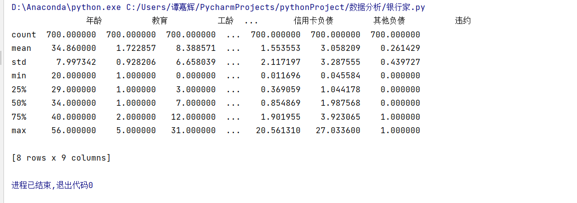
#从bankloan.xls中读取数据
data_load = "work/bankloan.xls"
data = pd.read_excel(data_load)
print(data.describe())

 

print(data.columns)
print(data.index)

 

 

 

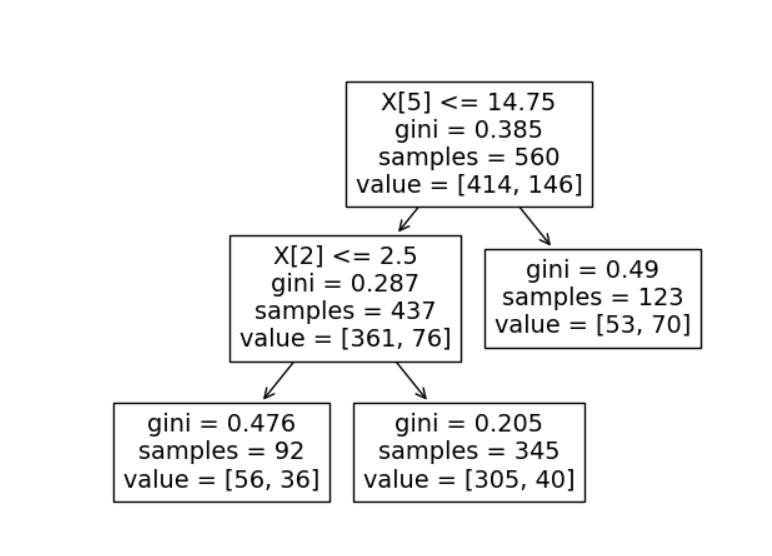
#生成决策树
X = np.array(data.iloc[:, 0:-1])
y = np.array(data.iloc[:, -1])

X_train, X_test, y_train, y_test = train_test_split(X, y, random_state=1, train_size=0.8, test_size=0.2, shuffle=True)


Dtree = DecisionTreeClassifier(max_leaf_nodes=3, random_state=13)
Dtree.fit(X_train, y_train)
y_pred = Dtree.predict(X_test)
accuracy_score(y_test, y_pred)

tree.plot_tree(Dtree)

plt.show()

 

 

 

 

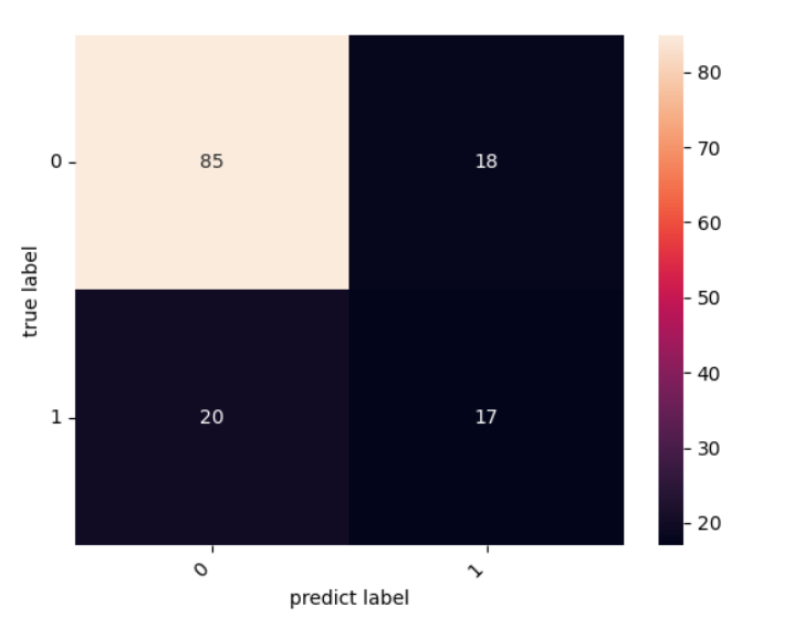
#混淆矩阵的可视化
cm = confusion_matrix(y_test, y_pred)
heatmap = sns.heatmap(cm, annot=True, fmt='d')
heatmap.yaxis.set_ticklabels(heatmap.yaxis.get_ticklabels(), rotation=0, ha='right')
heatmap.xaxis.set_ticklabels(heatmap.xaxis.get_ticklabels(), rotation=45, ha='right')
plt.ylabel("true label")
plt.xlabel("predict label")
plt.show()

 

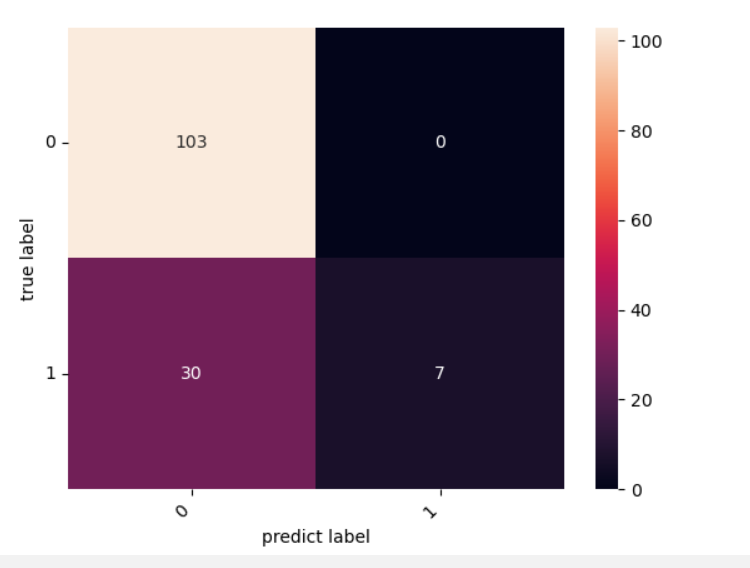
#svm支持向量机
svm = svm.SVC()

svm.fit(X_test,y_test)

y_pred = svm.predict(X_test)

accuracy_score(y_test, y_pred)

 

 

 

 

cm = confusion_matrix(y_test, y_pred)
heatmap = sns.heatmap(cm, annot=True, fmt='d')
heatmap.yaxis.set_ticklabels(heatmap.yaxis.get_ticklabels(), rotation=0, ha='right')
heatmap.xaxis.set_ticklabels(heatmap.xaxis.get_ticklabels(), rotation=45, ha='right')
plt.ylabel("true label")
plt.xlabel("predict label")
plt.show()

 

 

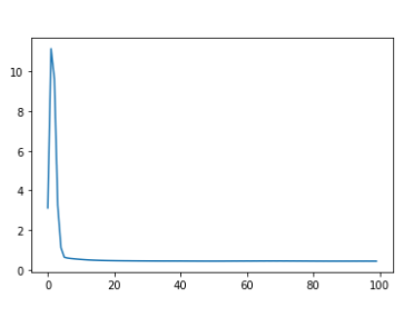
import torch
import torch.nn.functional as Fun
train_x = torch.FloatTensor(X_train)
train_y = torch.LongTensor(y_train)
test_x = torch.FloatTensor(X_test)
test_y = torch.LongTensor(y_test)
class Net(torch.nn.Module):
def __init__(self, n_feature, n_hidden, n_output):
super(Net, self).__init__()
self.hidden = torch.nn.Linear(n_feature, n_hidden) # 定义隐藏层网络
self.out = torch.nn.Linear(n_hidden, n_output) # 定义输出层网络

def forward(self, x):
x = Fun.relu(self.hidden(x)) # 隐藏层的激活函数,采用relu,也可以采用sigmod,tanh
x = self.out(x) # 输出层不用激活函数
return x

net = Net(n_feature=8,n_hidden=20, n_output=2) #n_feature:输入的特征维度,n_hiddenb:神经元个数,n_output:输出的类别个数
optimizer = torch.optim.SGD(net.parameters(), lr=0.02) # 优化器选用随机梯度下降方式
loss_func = torch.nn.CrossEntropyLoss() # 交叉熵损失函数
loss_record = []
for t in range(100):
out = net(train_x) # 输入input,输出out
loss = loss_func(out, train_y) # 输出与label对比
loss_record.append(loss.item())
optimizer.zero_grad() # 梯度清零
loss.backward() # 前馈操作
optimizer.step() # 使用梯度优化器
out = net(test_x) #out是一个计算矩阵，可以用Fun.softmax(out)转化为概率矩阵
prediction = torch.max(out, 1)[1] # 返回index 0返回原值
pred_y = prediction.data.numpy()
target_y = test_y.data.numpy()
accuracy = float((pred_y == target_y).astype(int).sum()) / float(target_y.size)
print(accuracy)
ax = sns.lineplot(data = loss_record)
plt.show()