BP-神经网络在fashion分类上的应用

# TensorFlow and tf.keras
import tensorflow as tf
from tensorflow import keras

# Helper libraries
import numpy as np
import matplotlib.pyplot as plt

print(tf.__version__)
fashion_mnist = keras.datasets.fashion_mnist

(train_images, train_labels), (test_images, test_labels) = fashion_mnist.load_data()
class_names = ['T-shirt/top', 'Trouser', 'Pullover', 'Dress', 'Coat',
               'Sandal', 'Shirt', 'Sneaker', 'Bag', 'Ankle boot']
train_images.shape
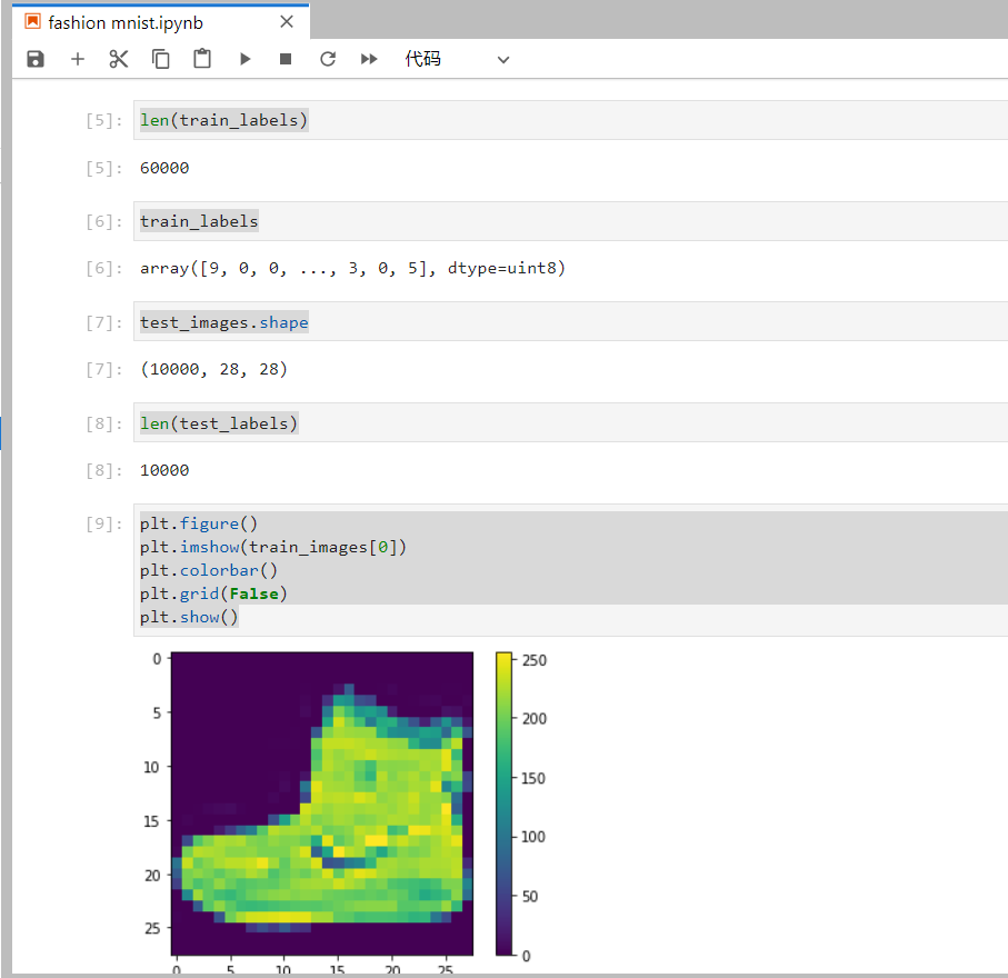
len(train_labels)
train_labels
test_images.shape
len(test_labels)
plt.figure()
plt.imshow(train_images[0])
plt.colorbar()
plt.grid(False)
plt.show()
train_images = train_images / 255.0

test_images = test_images / 255.0
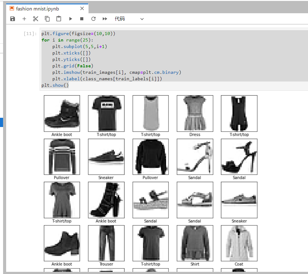
plt.figure(figsize=(10,10))
for i in range(25):
    plt.subplot(5,5,i+1)
    plt.xticks([])
    plt.yticks([])
    plt.grid(False)
    plt.imshow(train_images[i], cmap=plt.cm.binary)
    plt.xlabel(class_names[train_labels[i]])
plt.show()
model = keras.Sequential([
    keras.layers.Flatten(input_shape=(28, 28)),
    keras.layers.Dense(128, activation='relu'),
    keras.layers.Dense(10)
])
model.compile(optimizer='adam',
              loss=tf.keras.losses.SparseCategoricalCrossentropy(from_logits=True),
              metrics=['accuracy'])
model.fit(train_images, train_labels, epochs=15)
test_loss, test_acc = model.evaluate(test_images,  test_labels, verbose=2)
accuracy
print('\nTest accuracy:', test_acc)
probability_model = tf.keras.Sequential([model, 
                                         tf.keras.layers.Softmax()])
predictions = probability_model.predict(test_images)
predictions[0]
np.argmax(predictions[0])
test_labels[0]
def plot_image(i, predictions_array, true_label, img):
  predictions_array, true_label, img = predictions_array, true_label[i], img[i]
  plt.grid(False)
  plt.xticks([])
  plt.yticks([])

  plt.imshow(img, cmap=plt.cm.binary)

  predicted_label = np.argmax(predictions_array)
  if predicted_label == true_label:
    color = 'blue'
  else:
    color = 'red'

  plt.xlabel("{} {:2.0f}% ({})".format(class_names[predicted_label],
                                100*np.max(predictions_array),
                                class_names[true_label]),
                                color=color)

def plot_value_array(i, predictions_array, true_label):
  predictions_array, true_label = predictions_array, true_label[i]
  plt.grid(False)
  plt.xticks(range(10))
  plt.yticks([])
  thisplot = plt.bar(range(10), predictions_array, color="#777777")
  plt.ylim([0, 1])
  predicted_label = np.argmax(predictions_array)

  thisplot[predicted_label].set_color('red')
  thisplot[true_label].set_color('blue')
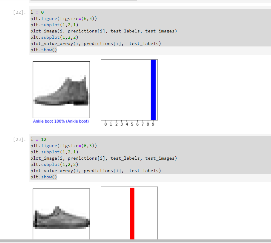
i = 0
plt.figure(figsize=(6,3))
plt.subplot(1,2,1)
plot_image(i, predictions[i], test_labels, test_images)
plt.subplot(1,2,2)
plot_value_array(i, predictions[i],  test_labels)
plt.show()
i = 12
plt.figure(figsize=(6,3))
plt.subplot(1,2,1)
plot_image(i, predictions[i], test_labels, test_images)
plt.subplot(1,2,2)
plot_value_array(i, predictions[i],  test_labels)
plt.show()
# Plot the first X test images, their predicted labels, and the true labels.
# Color correct predictions in blue and incorrect predictions in red.
num_rows = 5
num_cols = 3
num_images = num_rows*num_cols
plt.figure(figsize=(2*2*num_cols, 2*num_rows))
for i in range(num_images):
  plt.subplot(num_rows, 2*num_cols, 2*i+1)
  plot_image(i, predictions[i], test_labels, test_images)
  plt.subplot(num_rows, 2*num_cols, 2*i+2)
  plot_value_array(i, predictions[i], test_labels)
plt.tight_layout()
plt.show()
# Grab an image from the test dataset.
img = test_images[1]

print(img.shape)
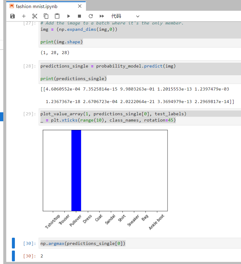
# Add the image to a batch where it's the only member.
img = (np.expand_dims(img,0))

print(img.shape)
predictions_single = probability_model.predict(img)

print(predictions_single)
plot_value_array(1, predictions_single[0], test_labels)
_ = plt.xticks(range(10), class_names, rotation=45)
np.argmax(predictions_single[0])