梯度下降法VS随机梯度下降法 (Python的实现)

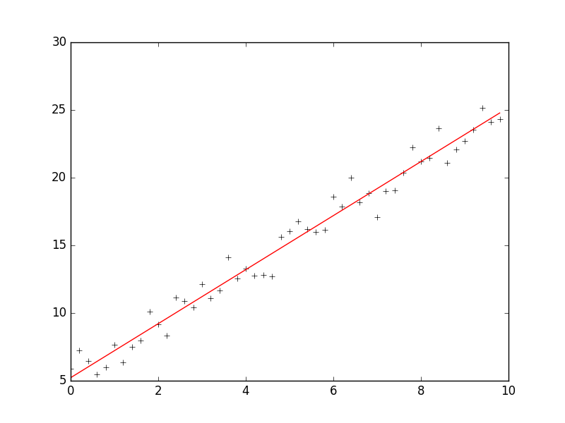
# -*- coding: cp936 -*-
import numpy as np
from scipy import stats
import matplotlib.pyplot as plt


# 构造训练数据
x = np.arange(0., 10., 0.2)
m = len(x)                                      # 训练数据点数目
x0 = np.full(m, 1.0)                 
input_data = np.vstack([x0, x]).T               # 将偏置b作为权向量的第一个分量
target_data = 2 * x + 5 + np.random.randn(m)


# 两种终止条件
loop_max = 10000   # 最大迭代次数(防止死循环)
epsilon = 1e-3     

# 初始化权值
np.random.seed(0)
w = np.random.randn(2)
#w = np.zeros(2)

alpha = 0.001      # 步长(注意取值过大会导致振荡,过小收敛速度变慢)
diff = 0.           
error = np.zeros(2) 
count = 0          # 循环次数
finish = 0         # 终止标志
# -------------------------------------------随机梯度下降算法----------------------------------------------------------
'''
while count < loop_max:
    count += 1

    # 遍历训练数据集，不断更新权值
    for i in range(m):  
        diff = np.dot(w, input_data[i]) - target_data[i]  # 训练集代入,计算误差值

        # 采用随机梯度下降算法,更新一次权值只使用一组训练数据
        w = w - alpha * diff * input_data[i]

        # ------------------------------终止条件判断-----------------------------------------
        # 若没终止，则继续读取样本进行处理，如果所有样本都读取完毕了,则循环重新从头开始读取样本进行处理。

    # ----------------------------------终止条件判断-----------------------------------------
    # 注意：有多种迭代终止条件，和判断语句的位置。终止判断可以放在权值向量更新一次后,也可以放在更新m次后。
    if np.linalg.norm(w - error) < epsilon:     # 终止条件：前后两次计算出的权向量的绝对误差充分小  
        finish = 1
        break
    else:
        error = w
print 'loop count = %d' % count,  '\tw:[%f, %f]' % (w[0], w[1])
'''


# -----------------------------------------------梯度下降法-----------------------------------------------------------
while count < loop_max:
    count += 1

    # 标准梯度下降是在权值更新前对所有样例汇总误差，而随机梯度下降的权值是通过考查某个训练样例来更新的
    # 在标准梯度下降中，权值更新的每一步对多个样例求和，需要更多的计算
    sum_m = np.zeros(2)
    for i in range(m):
        dif = (np.dot(w, input_data[i]) - target_data[i]) * input_data[i]
        sum_m = sum_m + dif     # 当alpha取值过大时,sum_m会在迭代过程中会溢出

    w = w - alpha * sum_m       # 注意步长alpha的取值,过大会导致振荡
    #w = w - 0.005 * sum_m      # alpha取0.005时产生振荡,需要将alpha调小
    
    # 判断是否已收敛
    if np.linalg.norm(w - error) < epsilon:
        finish = 1
        break
    else:
        error = w
print 'loop count = %d' % count,  '\tw:[%f, %f]' % (w[0], w[1])

# check with scipy linear regression 
slope, intercept, r_value, p_value, slope_std_error = stats.linregress(x, target_data)
print 'intercept = %s slope = %s' %(intercept, slope)
    
plt.plot(x, target_data, 'k+')
plt.plot(x, w[1] * x + w[0], 'r')
plt.show()

 

 

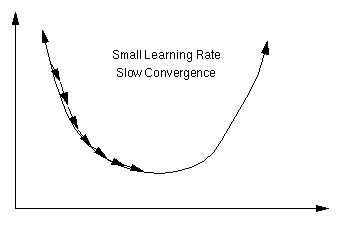
The Learning Rate

An important consideration is the learning rate µ, which determines by how much we change the weights w at each step. If µ is too small, the algorithm will take a long time to converge .

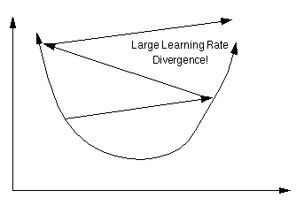
Conversely, if µ is too large, we may end up bouncing around the error surface out of control - the algorithm diverges. This usually ends with an overflow error in the computer's floating-point arithmetic.

 

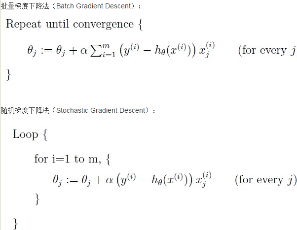
Batch vs. Online Learning

Above we have accumulated the gradient contributions for all data points in the training set before updating the weights. This method is often referred to as batch learning. An alternative approach is online learning, where the weights are updated immediately after seeing each data point. Since the gradient for a single data point can be considered a noisy approximation to the overall gradient, this is also called stochastic gradient descent.

Online learning has a number of advantages:

• it is often much faster, especially when the training set is redundant (contains many similar data points),
• it can be used when there is no fixed training set (new data keeps coming in),
• it is better at tracking nonstationary environments (where the best model gradually changes over time),
• the noise in the gradient can help to escape from local minima (which are a problem for gradient descent in nonlinear models)

These advantages are, however, bought at a price: many powerful optimization techniques (such as: conjugate and second-order gradient methods, support vector machines, Bayesian methods, etc.)  are batch methods that cannot be used online.A compromise between batch and online learning is the use of "mini-batches": the weights are updated after every n data points, where n is greater than 1 but smaller than the training set size.

 

 

参考：http://www.tuicool.com/articles/MRbee2i

     https://www.willamette.edu/~gorr/classes/cs449/linear2.html

     http://www.bogotobogo.com/python/python_numpy_batch_gradient_descent_algorithm.php