
griddata二维插值
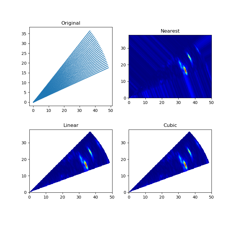
对某些设备或测量仪器来说,采集的数据点的位置不是规则排列的网格结构(可参考VTK基本数据结构),对于这种数据用散点图(每个采样点具有不同的值或权重)不能很好的展示其内部结构,因此需要对其进行插值,生成一个规则的栅格图像。可采用griddata函数对已知的数据点进行插值,数据点(X, Y)不要求规则排列。下图分别使用Nearest、Linear、Cubic三种插值方法对数据点进行插值。
插值算法都要首先面对一个共同的问题—— 邻近点的选择(利用靠近插值点附近的多个邻近点,构造插值函数计算插值点的函数值)。应尽可能使所选择的邻近点均匀地分布在待估点周围 。因为使用适量的已知点对于插值的精度很重要,当已知点过多时,会使插值准确率下降,因为过多的信息量会掩盖有用的信息;被选择的邻近点构成的点分布不均匀,若某个方位上的数据点过多,或点集的某些数据点位置较集中,或者数据点过远,都会带来较大的插值误差。griddata函数内部会先对已知的数据点进行Delaunay三角剖分,当完成三角剖分完成后,根据每个三角片顶点的数值,就可以对三角形区域内任意点进行线性插值(参考LinearNDInterpolator函数)。对三角片内的插值点可采用质心插值,即是对插值点只考虑与该点最邻近周围点的影响,确定出插值点与最邻近的周围点之相互位置关系,求出与周围点的影响权重因子,以此建立线性插值公式(参考重心坐标Barycentric coordinates)。


""" Simple N-D interpolation .. versionadded:: 0.9 """ # # Copyright (C) Pauli Virtanen, 2010. # # Distributed under the same BSD license as Scipy. # # # Note: this file should be run through the Mako template engine before # feeding it to Cython. # # Run ``generate_qhull.py`` to regenerate the ``qhull.c`` file # cimport cython from libc.float cimport DBL_EPSILON from libc.math cimport fabs, sqrt import numpy as np import scipy.spatial.qhull as qhull cimport scipy.spatial.qhull as qhull import warnings #------------------------------------------------------------------------------ # Numpy etc. #------------------------------------------------------------------------------ cdef extern from "numpy/ndarrayobject.h": cdef enum: NPY_MAXDIMS ctypedef fused double_or_complex: double double complex #------------------------------------------------------------------------------ # Interpolator base class #------------------------------------------------------------------------------ class NDInterpolatorBase(object): """ Common routines for interpolators. .. versionadded:: 0.9 """ def __init__(self, points, values, fill_value=np.nan, ndim=None, rescale=False, need_contiguous=True, need_values=True): """ Check shape of points and values arrays, and reshape values to (npoints, nvalues). Ensure the `points` and values arrays are C-contiguous, and of correct type. """ if isinstance(points, qhull.Delaunay): # Precomputed triangulation was passed in if rescale: raise ValueError("Rescaling is not supported when passing " "a Delaunay triangulation as ``points``.") self.tri = points points = points.points else: self.tri = None points = _ndim_coords_from_arrays(points) values = np.asarray(values) _check_init_shape(points, values, ndim=ndim) if need_contiguous: points = np.ascontiguousarray(points, dtype=np.double) if need_values: self.values_shape = values.shape[1:] if values.ndim == 1: self.values = values[:,None] elif values.ndim == 2: self.values = values else: self.values = values.reshape(values.shape[0], np.prod(values.shape[1:])) # Complex or real? self.is_complex = np.issubdtype(self.values.dtype, np.complexfloating) if self.is_complex: if need_contiguous: self.values = np.ascontiguousarray(self.values, dtype=np.complex128) self.fill_value = complex(fill_value) else: if need_contiguous: self.values = np.ascontiguousarray(self.values, dtype=np.double) self.fill_value = float(fill_value) if not rescale: self.scale = None self.points = points else: # scale to unit cube centered at 0 self.offset = np.mean(points, axis=0) self.points = points - self.offset self.scale = self.points.ptp(axis=0) self.scale[~(self.scale > 0)] = 1.0 # avoid division by 0 self.points /= self.scale def _check_call_shape(self, xi): xi = np.asanyarray(xi) if xi.shape[-1] != self.points.shape[1]: raise ValueError("number of dimensions in xi does not match x") return xi def _scale_x(self, xi): if self.scale is None: return xi else: return (xi - self.offset) / self.scale def __call__(self, *args): """ interpolator(xi) Evaluate interpolator at given points. Parameters ---------- x1, x2, ... xn: array-like of float Points where to interpolate data at. x1, x2, ... xn can be array-like of float with broadcastable shape. or x1 can be array-like of float with shape ``(..., ndim)`` """ xi = _ndim_coords_from_arrays(args, ndim=self.points.shape[1]) xi = self._check_call_shape(xi) shape = xi.shape xi = xi.reshape(-1, shape[-1]) xi = np.ascontiguousarray(xi, dtype=np.double) xi = self._scale_x(xi) if self.is_complex: r = self._evaluate_complex(xi) else: r = self._evaluate_double(xi) return np.asarray(r).reshape(shape[:-1] + self.values_shape) cpdef _ndim_coords_from_arrays(points, ndim=None): """ Convert a tuple of coordinate arrays to a (..., ndim)-shaped array. """ cdef ssize_t j, n if isinstance(points, tuple) and len(points) == 1: # handle argument tuple points = points[0] if isinstance(points, tuple): p = np.broadcast_arrays(*points) n = len(p) for j in range(1, n): if p[j].shape != p[0].shape: raise ValueError("coordinate arrays do not have the same shape") points = np.empty(p[0].shape + (len(points),), dtype=float) for j, item in enumerate(p): points[...,j] = item else: points = np.asanyarray(points) if points.ndim == 1: if ndim is None: points = points.reshape(-1, 1) else: points = points.reshape(-1, ndim) return points cdef _check_init_shape(points, values, ndim=None): """ Check shape of points and values arrays """ if values.shape[0] != points.shape[0]: raise ValueError("different number of values and points") if points.ndim != 2: raise ValueError("invalid shape for input data points") if points.shape[1] < 2: raise ValueError("input data must be at least 2-D") if ndim is not None and points.shape[1] != ndim: raise ValueError("this mode of interpolation available only for " "%d-D data" % ndim) #------------------------------------------------------------------------------ # Linear interpolation in N-D #------------------------------------------------------------------------------ class LinearNDInterpolator(NDInterpolatorBase): """ LinearNDInterpolator(points, values, fill_value=np.nan, rescale=False) Piecewise linear interpolant in N dimensions. .. versionadded:: 0.9 Methods ------- __call__ Parameters ---------- points : ndarray of floats, shape (npoints, ndims); or Delaunay Data point coordinates, or a precomputed Delaunay triangulation. values : ndarray of float or complex, shape (npoints, ...) Data values. fill_value : float, optional Value used to fill in for requested points outside of the convex hull of the input points. If not provided, then the default is ``nan``. rescale : bool, optional Rescale points to unit cube before performing interpolation. This is useful if some of the input dimensions have incommensurable units and differ by many orders of magnitude. Notes ----- The interpolant is constructed by triangulating the input data with Qhull [1]_, and on each triangle performing linear barycentric interpolation. Examples -------- We can interpolate values on a 2D plane: >>> from scipy.interpolate import LinearNDInterpolator >>> import matplotlib.pyplot as plt >>> np.random.seed(0) >>> x = np.random.random(10) - 0.5 >>> y = np.random.random(10) - 0.5 >>> z = np.hypot(x, y) >>> X = np.linspace(min(x), max(x)) >>> Y = np.linspace(min(y), max(y)) >>> X, Y = np.meshgrid(X, Y) # 2D grid for interpolation >>> interp = LinearNDInterpolator(list(zip(x, y)), z) >>> Z = interp(X, Y) >>> plt.pcolormesh(X, Y, Z, shading='auto') >>> plt.plot(x, y, "ok", label="input point") >>> plt.legend() >>> plt.colorbar() >>> plt.axis("equal") >>> plt.show() See also -------- griddata : Interpolate unstructured D-D data. NearestNDInterpolator : Nearest-neighbor interpolation in N dimensions. CloughTocher2DInterpolator : Piecewise cubic, C1 smooth, curvature-minimizing interpolant in 2D. References ---------- .. [1] http://www.qhull.org/ """ def __init__(self, points, values, fill_value=np.nan, rescale=False): NDInterpolatorBase.__init__(self, points, values, fill_value=fill_value, rescale=rescale) if self.tri is None: self.tri = qhull.Delaunay(self.points) def _evaluate_double(self, xi): return self._do_evaluate(xi, 1.0) def _evaluate_complex(self, xi): return self._do_evaluate(xi, 1.0j) @cython.boundscheck(False) @cython.wraparound(False) def _do_evaluate(self, const double[:,::1] xi, double_or_complex dummy): cdef const double_or_complex[:,::1] values = self.values cdef double_or_complex[:,::1] out cdef const double[:,::1] points = self.points cdef const int[:,::1] simplices = self.tri.simplices cdef double c[NPY_MAXDIMS] cdef double_or_complex fill_value cdef int i, j, k, m, ndim, isimplex, inside, start, nvalues cdef qhull.DelaunayInfo_t info cdef double eps, eps_broad ndim = xi.shape[1] start = 0 fill_value = self.fill_value qhull._get_delaunay_info(&info, self.tri, 1, 0, 0) out = np.empty((xi.shape[0], self.values.shape[1]), dtype=self.values.dtype) nvalues = out.shape[1] eps = 100 * DBL_EPSILON eps_broad = sqrt(DBL_EPSILON) with nogil: for i in range(xi.shape[0]): # 1) Find the simplex isimplex = qhull._find_simplex(&info, c, &xi[0,0] + i*ndim, &start, eps, eps_broad) # 2) Linear barycentric interpolation if isimplex == -1: # don't extrapolate for k in range(nvalues): out[i,k] = fill_value continue for k in range(nvalues): out[i,k] = 0 for j in range(ndim+1): for k in range(nvalues): m = simplices[isimplex,j] out[i,k] = out[i,k] + c[j] * values[m,k] return out #------------------------------------------------------------------------------ # Gradient estimation in 2D #------------------------------------------------------------------------------ class GradientEstimationWarning(Warning): pass @cython.cdivision(True) cdef int _estimate_gradients_2d_global(qhull.DelaunayInfo_t *d, double *data, int maxiter, double tol, double *y) nogil: """ Estimate gradients of a function at the vertices of a 2d triangulation. Parameters ---------- info : input Triangulation in 2D data : input Function values at the vertices maxiter : input Maximum number of Gauss-Seidel iterations tol : input Absolute / relative stop tolerance y : output, shape (npoints, 2) Derivatives [F_x, F_y] at the vertices Returns ------- num_iterations Number of iterations if converged, 0 if maxiter reached without convergence Notes ----- This routine uses a re-implementation of the global approximate curvature minimization algorithm described in [Nielson83] and [Renka84]. References ---------- .. [Nielson83] G. Nielson, ''A method for interpolating scattered data based upon a minimum norm network''. Math. Comp., 40, 253 (1983). .. [Renka84] R. J. Renka and A. K. Cline. ''A Triangle-based C1 interpolation method.'', Rocky Mountain J. Math., 14, 223 (1984). """ cdef double Q[2*2] cdef double s[2] cdef double r[2] cdef int ipoint, iiter, k, ipoint2, jpoint2 cdef double f1, f2, df2, ex, ey, L, L3, det, err, change # initialize for ipoint in range(2*d.npoints): y[ipoint] = 0 # # Main point: # # Z = sum_T sum_{E in T} int_E |W''|^2 = min! # # where W'' is the second derivative of the Clough-Tocher # interpolant to the direction of the edge E in triangle T. # # The minimization is done iteratively: for each vertex V, # the sum # # Z_V = sum_{E connected to V} int_E |W''|^2 # # is minimized separately, using existing values at other V. # # Since the interpolant can be written as # # W(x) = f(x) + w(x)^T y # # where y = [ F_x(V); F_y(V) ], it is clear that the solution to # the local problem is is given as a solution of the 2x2 matrix # equation. # # Here, we use the Clough-Tocher interpolant, which restricted to # a single edge is # # w(x) = (1 - x)**3 * f1 # + x*(1 - x)**2 * (df1 + 3*f1) # + x**2*(1 - x) * (df2 + 3*f2) # + x**3 * f2 # # where f1, f2 are values at the vertices, and df1 and df2 are # derivatives along the edge (away from the vertices). # # As a consequence, one finds # # L^3 int_{E} |W''|^2 = y^T A y + 2 B y + C # # with # # A = [4, -2; -2, 4] # B = [6*(f1 - f2), 6*(f2 - f1)] # y = [df1, df2] # L = length of edge E # # and C is not needed for minimization. Since df1 = dF1.E, df2 = -dF2.E, # with dF1 = [F_x(V_1), F_y(V_1)], and the edge vector E = V2 - V1, # we have # # Z_V = dF1^T Q dF1 + 2 s.dF1 + const. # # which is minimized by # # dF1 = -Q^{-1} s # # where # # Q = sum_E [A_11 E E^T]/L_E^3 = 4 sum_E [E E^T]/L_E^3 # s = sum_E [ B_1 + A_21 df2] E /L_E^3 # = sum_E [ 6*(f1 - f2) + 2*(E.dF2)] E / L_E^3 # # Gauss-Seidel for iiter in range(maxiter): err = 0 for ipoint in range(d.npoints): for k in range(2*2): Q[k] = 0 for k in range(2): s[k] = 0 # walk over neighbours of given point for jpoint2 in range(d.vertex_neighbors_indptr[ipoint], d.vertex_neighbors_indptr[ipoint+1]): ipoint2 = d.vertex_neighbors_indices[jpoint2] # edge ex = d.points[2*ipoint2 + 0] - d.points[2*ipoint + 0] ey = d.points[2*ipoint2 + 1] - d.points[2*ipoint + 1] L = sqrt(ex**2 + ey**2) L3 = L*L*L # data at vertices f1 = data[ipoint] f2 = data[ipoint2] # scaled gradient projections on the edge df2 = -ex*y[2*ipoint2 + 0] - ey*y[2*ipoint2 + 1] # edge sum Q[0] += 4*ex*ex / L3 Q[1] += 4*ex*ey / L3 Q[3] += 4*ey*ey / L3 s[0] += (6*(f1 - f2) - 2*df2) * ex / L3 s[1] += (6*(f1 - f2) - 2*df2) * ey / L3 Q[2] = Q[1] # solve det = Q[0]*Q[3] - Q[1]*Q[2] r[0] = ( Q[3]*s[0] - Q[1]*s[1])/det r[1] = (-Q[2]*s[0] + Q[0]*s[1])/det change = max(fabs(y[2*ipoint + 0] + r[0]), fabs(y[2*ipoint + 1] + r[1])) y[2*ipoint + 0] = -r[0] y[2*ipoint + 1] = -r[1] # relative/absolute error change /= max(1.0, max(fabs(r[0]), fabs(r[1]))) err = max(err, change) if err < tol: return iiter + 1 # Didn't converge before maxiter return 0 @cython.boundscheck(False) @cython.wraparound(False) cpdef estimate_gradients_2d_global(tri, y, int maxiter=400, double tol=1e-6): cdef const double[:,::1] data cdef double[:,:,::1] grad cdef qhull.DelaunayInfo_t info cdef int k, ret, nvalues y = np.asanyarray(y) if y.shape[0] != tri.npoints: raise ValueError("'y' has a wrong number of items") if np.issubdtype(y.dtype, np.complexfloating): rg = estimate_gradients_2d_global(tri, y.real, maxiter=maxiter, tol=tol) ig = estimate_gradients_2d_global(tri, y.imag, maxiter=maxiter, tol=tol) r = np.zeros(rg.shape, dtype=complex) r.real = rg r.imag = ig return r y_shape = y.shape if y.ndim == 1: y = y[:,None] y = y.reshape(tri.npoints, -1).T y = np.ascontiguousarray(y, dtype=np.double) yi = np.empty((y.shape[0], y.shape[1], 2)) data = y grad = yi qhull._get_delaunay_info(&info, tri, 0, 0, 1) nvalues = data.shape[0] for k in range(nvalues): with nogil: ret = _estimate_gradients_2d_global( &info, &data[k,0], maxiter, tol, &grad[k,0,0]) if ret == 0: warnings.warn("Gradient estimation did not converge, " "the results may be inaccurate", GradientEstimationWarning) return yi.transpose(1, 0, 2).reshape(y_shape + (2,)) #------------------------------------------------------------------------------ # Cubic interpolation in 2D #------------------------------------------------------------------------------ @cython.cdivision(True) cdef double_or_complex _clough_tocher_2d_single(qhull.DelaunayInfo_t *d, int isimplex, double *b, double_or_complex *f, double_or_complex *df) nogil: """ Evaluate Clough-Tocher interpolant on a 2D triangle. Parameters ---------- d : Delaunay info isimplex : int Triangle to evaluate on b : shape (3,) Barycentric coordinates of the point on the triangle f : shape (3,) Function values at vertices df : shape (3, 2) Gradient values at vertices Returns ------- w : Value of the interpolant at the given point References ---------- .. [CT] See, for example, P. Alfeld, ''A trivariate Clough-Tocher scheme for tetrahedral data''. Computer Aided Geometric Design, 1, 169 (1984); G. Farin, ''Triangular Bernstein-Bezier patches''. Computer Aided Geometric Design, 3, 83 (1986). """ cdef double_or_complex \ c3000, c0300, c0030, c0003, \ c2100, c2010, c2001, c0210, c0201, c0021, \ c1200, c1020, c1002, c0120, c0102, c0012, \ c1101, c1011, c0111 cdef double_or_complex \ f1, f2, f3, df12, df13, df21, df23, df31, df32 cdef double g[3] cdef double \ e12x, e12y, e23x, e23y, e31x, e31y, \ e14x, e14y, e24x, e24y, e34x, e34y cdef double_or_complex w cdef double minval cdef double b1, b2, b3, b4 cdef int k, itri cdef double c[3] cdef double y[2] # XXX: optimize + refactor this! e12x = (+ d.points[0 + 2*d.simplices[3*isimplex + 1]] - d.points[0 + 2*d.simplices[3*isimplex + 0]]) e12y = (+ d.points[1 + 2*d.simplices[3*isimplex + 1]] - d.points[1 + 2*d.simplices[3*isimplex + 0]]) e23x = (+ d.points[0 + 2*d.simplices[3*isimplex + 2]] - d.points[0 + 2*d.simplices[3*isimplex + 1]]) e23y = (+ d.points[1 + 2*d.simplices[3*isimplex + 2]] - d.points[1 + 2*d.simplices[3*isimplex + 1]]) e31x = (+ d.points[0 + 2*d.simplices[3*isimplex + 0]] - d.points[0 + 2*d.simplices[3*isimplex + 2]]) e31y = (+ d.points[1 + 2*d.simplices[3*isimplex + 0]] - d.points[1 + 2*d.simplices[3*isimplex + 2]]) e14x = (e12x - e31x)/3 e14y = (e12y - e31y)/3 e24x = (-e12x + e23x)/3 e24y = (-e12y + e23y)/3 e34x = (e31x - e23x)/3 e34y = (e31y - e23y)/3 f1 = f[0] f2 = f[1] f3 = f[2] df12 = +(df[2*0+0]*e12x + df[2*0+1]*e12y) df21 = -(df[2*1+0]*e12x + df[2*1+1]*e12y) df23 = +(df[2*1+0]*e23x + df[2*1+1]*e23y) df32 = -(df[2*2+0]*e23x + df[2*2+1]*e23y) df31 = +(df[2*2+0]*e31x + df[2*2+1]*e31y) df13 = -(df[2*0+0]*e31x + df[2*0+1]*e31y) c3000 = f1 c2100 = (df12 + 3*c3000)/3 c2010 = (df13 + 3*c3000)/3 c0300 = f2 c1200 = (df21 + 3*c0300)/3 c0210 = (df23 + 3*c0300)/3 c0030 = f3 c1020 = (df31 + 3*c0030)/3 c0120 = (df32 + 3*c0030)/3 c2001 = (c2100 + c2010 + c3000)/3 c0201 = (c1200 + c0300 + c0210)/3 c0021 = (c1020 + c0120 + c0030)/3 # # Now, we need to impose the condition that the gradient of the spline # to some direction `w` is a linear function along the edge. # # As long as two neighbouring triangles agree on the choice of the # direction `w`, this ensures global C1 differentiability. # Otherwise, the choice of the direction is arbitrary (except that # it should not point along the edge, of course). # # In [CT]_, it is suggested to pick `w` as the normal of the edge. # This choice is given by the formulas # # w_12 = E_24 + g[0] * E_23 # w_23 = E_34 + g[1] * E_31 # w_31 = E_14 + g[2] * E_12 # # g[0] = -(e24x*e23x + e24y*e23y) / (e23x**2 + e23y**2) # g[1] = -(e34x*e31x + e34y*e31y) / (e31x**2 + e31y**2) # g[2] = -(e14x*e12x + e14y*e12y) / (e12x**2 + e12y**2) # # However, this choice gives an interpolant that is *not* # invariant under affine transforms. This has some bad # consequences: for a very narrow triangle, the spline can # develops huge oscillations. For instance, with the input data # # [(0, 0), (0, 1), (eps, eps)], eps = 0.01 # F = [0, 0, 1] # dF = [(0,0), (0,0), (0,0)] # # one observes that as eps -> 0, the absolute maximum value of the # interpolant approaches infinity. # # So below, we aim to pick affine invariant `g[k]`. # We choose # # w = V_4' - V_4 # # where V_4 is the centroid of the current triangle, and V_4' the # centroid of the neighbour. Since this quantity transforms similarly # as the gradient under affine transforms, the resulting interpolant # is affine-invariant. Moreover, two neighbouring triangles clearly # always agree on the choice of `w` (sign is unimportant), and so # this choice also makes the interpolant C1. # # The drawback here is a performance penalty, since we need to # peek into neighbouring triangles. # for k in range(3): itri = d.neighbors[3*isimplex + k] if itri == -1: # No neighbour. # Compute derivative to the centroid direction (e_12 + e_13)/2. g[k] = -1./2 continue # Centroid of the neighbour, in our local barycentric coordinates y[0] = (+ d.points[0 + 2*d.simplices[3*itri + 0]] + d.points[0 + 2*d.simplices[3*itri + 1]] + d.points[0 + 2*d.simplices[3*itri + 2]]) / 3 y[1] = (+ d.points[1 + 2*d.simplices[3*itri + 0]] + d.points[1 + 2*d.simplices[3*itri + 1]] + d.points[1 + 2*d.simplices[3*itri + 2]]) / 3 qhull._barycentric_coordinates(2, d.transform + isimplex*2*3, y, c) # Rewrite V_4'-V_4 = const*[(V_4-V_2) + g_i*(V_3 - V_2)] # Now, observe that the results can be written *in terms of # barycentric coordinates*. Barycentric coordinates stay # invariant under affine transformations, so we can directly # conclude that the choice below is affine-invariant. if k == 0: g[k] = (2*c[2] + c[1] - 1) / (2 - 3*c[2] - 3*c[1]) elif k == 1: g[k] = (2*c[0] + c[2] - 1) / (2 - 3*c[0] - 3*c[2]) elif k == 2: g[k] = (2*c[1] + c[0] - 1) / (2 - 3*c[1] - 3*c[0]) c0111 = (g[0]*(-c0300 + 3*c0210 - 3*c0120 + c0030) + (-c0300 + 2*c0210 - c0120 + c0021 + c0201))/2 c1011 = (g[1]*(-c0030 + 3*c1020 - 3*c2010 + c3000) + (-c0030 + 2*c1020 - c2010 + c2001 + c0021))/2 c1101 = (g[2]*(-c3000 + 3*c2100 - 3*c1200 + c0300) + (-c3000 + 2*c2100 - c1200 + c2001 + c0201))/2 c1002 = (c1101 + c1011 + c2001)/3 c0102 = (c1101 + c0111 + c0201)/3 c0012 = (c1011 + c0111 + c0021)/3 c0003 = (c1002 + c0102 + c0012)/3 # extended barycentric coordinates minval = b[0] for k in range(3): if b[k] < minval: minval = b[k] b1 = b[0] - minval b2 = b[1] - minval b3 = b[2] - minval b4 = 3*minval # evaluate the polynomial -- the stupid and ugly way to do it, # one of the 4 coordinates is in fact zero w = (b1**3*c3000 + 3*b1**2*b2*c2100 + 3*b1**2*b3*c2010 + 3*b1**2*b4*c2001 + 3*b1*b2**2*c1200 + 6*b1*b2*b4*c1101 + 3*b1*b3**2*c1020 + 6*b1*b3*b4*c1011 + 3*b1*b4**2*c1002 + b2**3*c0300 + 3*b2**2*b3*c0210 + 3*b2**2*b4*c0201 + 3*b2*b3**2*c0120 + 6*b2*b3*b4*c0111 + 3*b2*b4**2*c0102 + b3**3*c0030 + 3*b3**2*b4*c0021 + 3*b3*b4**2*c0012 + b4**3*c0003) return w class CloughTocher2DInterpolator(NDInterpolatorBase): """ CloughTocher2DInterpolator(points, values, tol=1e-6) Piecewise cubic, C1 smooth, curvature-minimizing interpolant in 2D. .. versionadded:: 0.9 Methods ------- __call__ Parameters ---------- points : ndarray of floats, shape (npoints, ndims); or Delaunay Data point coordinates, or a precomputed Delaunay triangulation. values : ndarray of float or complex, shape (npoints, ...) Data values. fill_value : float, optional Value used to fill in for requested points outside of the convex hull of the input points. If not provided, then the default is ``nan``. tol : float, optional Absolute/relative tolerance for gradient estimation. maxiter : int, optional Maximum number of iterations in gradient estimation. rescale : bool, optional Rescale points to unit cube before performing interpolation. This is useful if some of the input dimensions have incommensurable units and differ by many orders of magnitude. Notes ----- The interpolant is constructed by triangulating the input data with Qhull [1]_, and constructing a piecewise cubic interpolating Bezier polynomial on each triangle, using a Clough-Tocher scheme [CT]_. The interpolant is guaranteed to be continuously differentiable. The gradients of the interpolant are chosen so that the curvature of the interpolating surface is approximatively minimized. The gradients necessary for this are estimated using the global algorithm described in [Nielson83]_ and [Renka84]_. Examples -------- We can interpolate values on a 2D plane: >>> from scipy.interpolate import CloughTocher2DInterpolator >>> import matplotlib.pyplot as plt >>> np.random.seed(0) >>> x = np.random.random(10) - 0.5 >>> y = np.random.random(10) - 0.5 >>> z = np.hypot(x, y) >>> X = np.linspace(min(x), max(x)) >>> Y = np.linspace(min(y), max(y)) >>> X, Y = np.meshgrid(X, Y) # 2D grid for interpolation >>> interp = CloughTocher2DInterpolator(list(zip(x, y)), z) >>> Z = interp(X, Y) >>> plt.pcolormesh(X, Y, Z, shading='auto') >>> plt.plot(x, y, "ok", label="input point") >>> plt.legend() >>> plt.colorbar() >>> plt.axis("equal") >>> plt.show() See also -------- griddata : Interpolate unstructured D-D data. LinearNDInterpolator : Piecewise linear interpolant in N dimensions. NearestNDInterpolator : Nearest-neighbor interpolation in N dimensions. References ---------- .. [1] http://www.qhull.org/ .. [CT] See, for example, P. Alfeld, ''A trivariate Clough-Tocher scheme for tetrahedral data''. Computer Aided Geometric Design, 1, 169 (1984); G. Farin, ''Triangular Bernstein-Bezier patches''. Computer Aided Geometric Design, 3, 83 (1986). .. [Nielson83] G. Nielson, ''A method for interpolating scattered data based upon a minimum norm network''. Math. Comp., 40, 253 (1983). .. [Renka84] R. J. Renka and A. K. Cline. ''A Triangle-based C1 interpolation method.'', Rocky Mountain J. Math., 14, 223 (1984). """ def __init__(self, points, values, fill_value=np.nan, tol=1e-6, maxiter=400, rescale=False): NDInterpolatorBase.__init__(self, points, values, ndim=2, fill_value=fill_value, rescale=rescale) if self.tri is None: self.tri = qhull.Delaunay(self.points) self.grad = estimate_gradients_2d_global(self.tri, self.values, tol=tol, maxiter=maxiter) def _evaluate_double(self, xi): return self._do_evaluate(xi, 1.0) def _evaluate_complex(self, xi): return self._do_evaluate(xi, 1.0j) @cython.boundscheck(False) @cython.wraparound(False) def _do_evaluate(self, const double[:,::1] xi, double_or_complex dummy): cdef const double_or_complex[:,::1] values = self.values cdef const double_or_complex[:,:,:] grad = self.grad cdef double_or_complex[:,::1] out cdef const double[:,::1] points = self.points cdef const int[:,::1] simplices = self.tri.simplices cdef double c[NPY_MAXDIMS] cdef double_or_complex f[NPY_MAXDIMS+1] cdef double_or_complex df[2*NPY_MAXDIMS+2] cdef double_or_complex w cdef double_or_complex fill_value cdef int i, j, k, m, ndim, isimplex, inside, start, nvalues cdef qhull.DelaunayInfo_t info cdef double eps, eps_broad ndim = xi.shape[1] start = 0 fill_value = self.fill_value qhull._get_delaunay_info(&info, self.tri, 1, 1, 0) out = np.zeros((xi.shape[0], self.values.shape[1]), dtype=self.values.dtype) nvalues = out.shape[1] eps = 100 * DBL_EPSILON eps_broad = sqrt(eps) with nogil: for i in range(xi.shape[0]): # 1) Find the simplex isimplex = qhull._find_simplex(&info, c, &xi[i,0], &start, eps, eps_broad) # 2) Clough-Tocher interpolation if isimplex == -1: # outside triangulation for k in range(nvalues): out[i,k] = fill_value continue for k in range(nvalues): for j in range(ndim+1): f[j] = values[simplices[isimplex,j],k] df[2*j] = grad[simplices[isimplex,j],k,0] df[2*j+1] = grad[simplices[isimplex,j],k,1] w = _clough_tocher_2d_single(&info, isimplex, c, f, df) out[i,k] = w return out
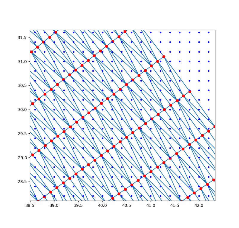
下图中红色的是已知采样点,蓝色是待插值的栅格点,三角形内部栅格点的数值可通过线性插值或其它插值方法计算出,三角形外部的点可在函数中指定一个数值(默认为NaN)。对于某些片层数据若采集的数据点位置不变,可以只计算一次Delaunay三角剖分,后续直接使用LinearNDInterpolator或CloughTocher2DInterpolator等函数进行插值,加快迭代计算的时间。
参考:
Interpolation (scipy.interpolate)
storing the weights used by scipy griddata for re-use
Speedup scipy griddata for multiple interpolations between two irregular grids

 浙公网安备 33010602011771号